A paper reports 50 steps to 4 and calls it a 12× speedup. Your service may not see 12×. This post is about the gap: the things you pay for besides network calls, the accelerations that cancel each other out, and the failure modes that only appear once the step count is low.
generative
diffusion
Published
August 1, 2026
The previous post showed how sampling can fall from dozens of denoiser evaluations to one to four. That may be a 12–50× reduction in NFE, but it is not automatically a 12–50× reduction in the latency a user sees.
The gap is not anyone being dishonest. It’s that NFE — the number of network evaluations — is a proxy for cost, and like all proxies it stops tracking the thing it stands for once you optimise it hard enough. This post is about what else you’re paying for, which accelerations cancel each other out, and the failure modes that only show up after the step count comes down.
TL;DR — NFE measures one part of a generation pipeline: denoiser work. As NFE falls, one-time costs such as text encoding, latent decoding, dispatch, and synchronization become visible; ordinary CFG roughly doubles denoiser-equivalent work; cross-step caching loses the redundancy it depends on; and approximation errors change character because there are fewer correction stages. In serving, predictable fixed-step execution can also beat a lower-average adaptive policy because batches stay aligned.
Where the time actually goes
Sampling is not the only thing a diffusion pipeline does. A text-to-image request may encode the prompt, prepare conditioning, and decode a latent into pixels. These are per-request or per-batch costs: they do not scale linearly with the number of denoising steps, although they still depend on batch size, resolution, model choice, and hardware.
In many conventional 50-step pipelines denoising dominates enough that these fixed costs receive little attention. It matters enormously at 4. The arithmetic is Amdahl’s law, and it’s worth doing explicitly because the intuition is unreliable:
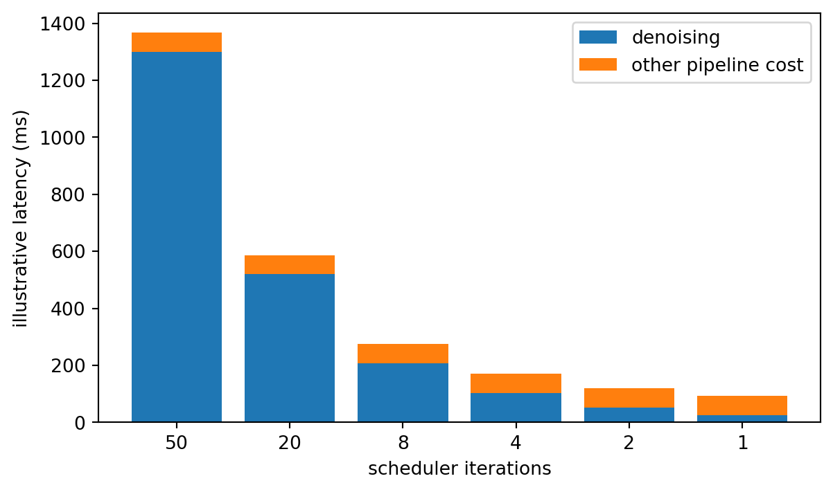
# Illustrative numbers for a text-to-image pipeline. The exact values depend# entirely on the model and hardware — what matters here is the SHAPE.text_encode =8.0# ms, once per requestper_step =26.0# ms, per denoising stepvae_decode =55.0# ms, once per requestoverhead =4.0# ms, scheduler + memory + dispatch, oncedef total_latency(steps):return text_encode + steps * per_step + vae_decode + overheadfor steps in [50, 20, 8, 4, 2, 1]: total = total_latency(steps) denoise_share = steps * per_step / totalprint(f"{steps:>3} steps: {total:>7.1f} ms "f"denoising is {denoise_share:>5.1%} of it "f"speedup vs 50 steps: {total_latency(50)/total:>5.2f}×")
 50 steps:  1367.0 ms   denoising is 95.1% of it   speedup vs 50 steps:  1.00×
 20 steps:   587.0 ms   denoising is 88.6% of it   speedup vs 50 steps:  2.33×
  8 steps:   275.0 ms   denoising is 75.6% of it   speedup vs 50 steps:  4.97×
  4 steps:   171.0 ms   denoising is 60.8% of it   speedup vs 50 steps:  7.99×
  2 steps:   119.0 ms   denoising is 43.7% of it   speedup vs 50 steps: 11.49×
  1 steps:    93.0 ms   denoising is 28.0% of it   speedup vs 50 steps: 14.70×
In this illustrative profile, going from 50 steps to 1 is a 50× reduction in NFE but only a 14.7× reduction in latency. The last stretch is especially inelastic: 4 steps to 1 cuts NFE by 4× and latency by only about 1.8×. At one step, denoising is 28% of this particular request.
Two practical consequences follow immediately:
Fixed costs can dominate surprisingly early. In the toy budget above, the decoder becomes larger than one denoising evaluation and dominates the one-step request. A larger DiT or a cheaper decoder can produce a very different crossover, so profile rather than memorise “eight steps.”
A one-step model is not automatically four times faster than a four-step model. The achievable ratio depends on the denoiser share, backbone size, CFG, decoder cost, batching, and kernel efficiency.
Code
import matplotlib.pyplot as pltstep_counts = [50, 20, 8, 4, 2, 1]denoise = [s * per_step for s in step_counts]fixed = [text_encode + vae_decode + overhead for _ in step_counts]plt.figure(figsize=(7, 4))plt.bar([str(s) for s in step_counts], denoise, label="denoising")plt.bar([str(s) for s in step_counts], fixed, bottom=denoise, label="other pipeline cost")plt.xlabel("scheduler iterations")plt.ylabel("illustrative latency (ms)")plt.legend()plt.show()
Illustrative latency decomposition. As denoising shrinks, one-time pipeline costs become the limiting fraction.
How to profile the real pipeline
The illustrative arithmetic is useful only if it leads to measurement. GPU timing has three common traps:
CUDA work is asynchronous, so ordinary wall-clock timing can stop before the kernels finish.
The first iterations include compilation, memory allocation, and cache warm-up.
End-to-end latency and isolated kernel time answer different questions.
A minimal harness should warm up, synchronize, repeat, and report the environment:
component time: text encoder, each denoiser call, VAE, and post-processing separately;
end-to-end time: the real request path, including transfers, synchronization, and batching.
Also record batch size, resolution, dtype, guidance mode, compilation state, hardware, and whether the reported number is cold, warm, p50, p95, latency, or saturated throughput. Without that context, a speedup is difficult to reproduce.
Guidance: the factor of two that goes uncounted
Classifier-free guidance is a common way to strengthen prompt conditioning. At each step it needs a conditional and an unconditional prediction. Implementations often concatenate both branches into one larger batch, so it may be one framework invocation, but it still performs roughly twice the denoiser arithmetic and uses more memory.
Twice. Every step.
steps =4print(f"a '{steps}-step' sampler with classifier-free guidance:")print(f" {steps} scheduler iterations")print(f" {steps} denoiser invocations, each with the batch doubled")print(f" ≈ {steps *2} single-branch evaluation equivalents of arithmetic")print()print("An unguided 8-step sampler has a similar single-branch FLOP count —")print("but not necessarily the same memory use or latency.")
a '4-step' sampler with classifier-free guidance:
   4 scheduler iterations
   4 denoiser invocations, each with the batch doubled
   ≈ 8 single-branch evaluation equivalents of arithmetic

An unguided 8-step sampler has a similar single-branch FLOP count —
but not necessarily the same memory use or latency.
For the same backbone, shape, and hardware, a four-step run with ordinary CFG performs roughly the denoiser work of eight unguided evaluations. Batching efficiency can change wall clock, so call this sample-equivalent denoiser work, not identical end-to-end cost. When step counts are compared, check whether guidance is inside or outside the accounting.
This also explains a behaviour that confuses people about distilled few-step models: some of them expect zero external CFG or a checkpoint-specific guidance range. Running ordinary CFG at one step would double the only denoiser work, so guidance is often distilled in — the student learns the already-guided output, sometimes with the guidance strength baked to a fixed value, sometimes as an extra input. Either way, the knob you’re turning is not the teacher’s knob, and it may have a much narrower useful range or none at all.
Caching: the speedup that vanishes exactly when you need it
Here’s an interaction that catches teams out.
Adjacent denoising steps produce very similar internal activations — the input barely changed, so much of the network’s intermediate work barely changed either. Cross-step feature caching exploits this: compute a block’s output at one step, reuse it for the next, skip the work. Methods like TeaCache and its relatives get substantial speedups this way, and it requires no retraining.
Now count what happens when you combine it with a few-step model:
for steps in [50, 20, 8, 4, 2, 1]: reuse_opportunities =max(steps -1, 0) # you can only reuse from a PREVIOUS stepprint(f"{steps:>3} steps → {reuse_opportunities:>2} chances to reuse a cached feature"f"{' ← nothing to cache'if reuse_opportunities ==0else''}")
 50 steps → 49 chances to reuse a cached feature
 20 steps → 19 chances to reuse a cached feature
  8 steps →  7 chances to reuse a cached feature
  4 steps →  3 chances to reuse a cached feature
  2 steps →  1 chances to reuse a cached feature
  1 steps →  0 chances to reuse a cached feature   ← nothing to cache
Cross-step caching and step reduction are not independent speedups—they compete for the same temporal redundancy. A 50-step sampler has enormous cross-step redundancy, which is why caching works so well there. A 1-step model has none, by construction. You cannot multiply the two speedups together, and a plan that assumes you can will overshoot badly.
The general lesson, which applies well beyond caching: acceleration techniques are not independent multipliers. Always measure the combination, never compose the individual claims.
Failure modes that become more consequential at low step counts
Six issues that are easier to tolerate, overlook, or repair at 50 steps than at 4.
1 · Your scheduler and your checkpoint disagree. Few-step models are trained for a specific sampling procedure. Loading a distilled checkpoint and running it with the default scheduler — or with a guidance scale it was never trained under — produces output that is bad in a way that looks like a bad model. Check what the checkpoint expects.
2 · A second-order label hides the real cost. A Runge–Kutta method such as Heun spends two fresh evaluations per step; a second-order multistep method may reuse a previous prediction and spend only one new call after startup. As the previous post measured, formal order can also reverse at extreme low NFE. Count new denoiser evaluations and validate the actual low-budget regime.
3 · Guidance applied twice. If guidance was distilled into the model and you also apply it at sampling time, you’re extrapolating an already-extrapolated prediction. The result can be oversaturation and posterised flat regions — the same signature as an over-cranked guidance scale, but arriving at a setting that looks reasonable.
4 · Prompt-conditioned diversity collapses while aggregate FID can look acceptable. Few-step models, especially adversarially trained ones, can lose sample variety. A distribution-level metric computed over thousands of prompts can look healthy while every image for a given prompt has become nearly identical. The check takes two minutes and almost nobody runs it: fix one prompt, vary the seed, look at the spread. Report that alongside FID.
5 · Pointwise distillation transfers the teacher’s behaviour. A student trained to reproduce the teacher’s seed-wise mapping will usually inherit systematic weaknesses—including schedule or terminal-SNR mismatch—unless auxiliary data or objectives counteract them. Distribution-level methods are less tightly anchored, which creates both room for improvement and room for drift.
6 · Approximation sensitivity changes when NFE changes. Quantization or cache error can accumulate across a long trajectory, but a multi-step sampler may also correct some imperfect intermediate states. A strict one-step generator has no later denoising stage in which to recover. There is no universal monotonic rule: revalidate precision, caching thresholds, and numerical approximations after changing NFE rather than inheriting the teacher’s settings.
Why adaptive step counts can lose in production
Adaptive solvers vary the number of steps per sample: easy samples finish early, hard ones get more. Offline that’s a clear win on average NFE.
In a serving system it frequently isn’t, and the two ways of implementing it fail differently:
Per-sample adaptivity fragments the batch. Different samples run different numbers of iterations, which means divergent execution and idle GPU while the stragglers finish.
A shared adaptive controller keeps the batch together but lets the hardest sample in it set the schedule for everyone.
Either can lose to a fixed four-step policy that batches predictably, even when the adaptive method uses fewer evaluations on average. This is a serving trade-off, not a universal result; the crossover depends on batch formation, workload variance, and whether the system can refill partially completed batches. The second failure is exactly the convoy effect from the continuous batching post, arriving in a different costume: a batch moves at the speed of its slowest member unless you design against it.
What’s actually worth doing
One reasonable decision order is below. The effort and useful NFE ranges are illustrative—they vary sharply with model size, data access, and infrastructure:
Approach
Cost to you
Typical NFE
Works on an existing model?
Compatible solver (DPM-Solver++, UniPC)
minimal
often 10–25
yes, when schedule and prediction type match
Tuned step placement (e.g. Align Your Steps)
search/evaluation
often 10–20
yes, for the model–solver pair
Optimise the decoder and fixed costs
hours
—
yes, and increasingly dominant
Feature caching
hours
10–50
yes, but conflicts with step reduction
Quantization
days
—
yes, revalidate at low NFE
LCM-LoRA style adapters
hours
4–8
yes, as an adapter
Distillation (DMD2, ADD, SiD)
substantial training
1–4
produces a new model
From-scratch one-step objective (MeanFlow family)
foundation-model training
1
no—it is the model
If you have a pretrained model and want it faster this week, the honest ordering is: exhaust the free options first (better solver, tuned step schedule), then measure where the time actually goes, and only then consider distillation. Teams routinely skip to distillation and discover afterwards that their VAE decoder was 40% of the latency.
One frontier note, briefly: recent work has started widening what “the budget” even means — 1.x-Distill explores fractional effective NFE with cache-aware distillation, and MrFlow stages low- and high-resolution sampling to cut spatial compute, composing with timestep distillation rather than replacing it. Both are recent preprints. They reinforce this post’s point: acceleration is not a single “number of steps” knob.
What to carry away
NFE is a proxy for cost, and it stops tracking cost once you optimise it hard. In the illustrative pipeline above, a 50× NFE reduction bought under 15× latency, and the final 4×-of-NFE bought about 1.8×.
Fixed costs can take over at low NFE. Their crossover is model- and hardware-specific; the only reliable answer comes from a component profile.
Ordinary CFG requires two predictions per step. They may be batched into one invocation, but the denoiser-equivalent work and memory pressure remain close to two branches.
Caching and step reduction eat the same redundancy. They do not multiply, and at one step there is nothing left to cache.
Revalidate approximations after changing NFE. Error may accumulate differently, and one-step models have no later correction stage.
Check per-prompt diversity, not just FID. Aggregate metrics hide the collapse that few-step models are most prone to.
Fixed schedules can beat adaptive ones in production when predictable batching matters more than a lower average NFE.
If one sentence survives: the number in the paper counts network evaluations, and the number in your latency budget counts everything else too.
Where this goes next
Three things this series deliberately left alone. Video, where every denoising evaluation processes many frames at once, so per-step compute and memory grow sharply with sequence length — which is what makes few-step generation the difference between a demo and a product. The systems layer — quantization, kernels, compilation and distributed inference — a complementary acceleration axis rather than an independent one, as the caching section above already shows, and often the cheapest win available. And flow matching itself, which has been used throughout as the convenient formalism without being derived properly; that derivation is its own post and the natural companion to this one.
References
Ma et al., DeepCache, 2023 — cross-step feature reuse, and the redundancy that few-step sampling removes.
Liu et al., TeaCache, 2024 — timestep-aware caching.
Li et al., SnapFusion, 2023 — an early and clear account of where the time actually goes in a diffusion pipeline.
Chen et al., SANA-Sprint, 2025 — few-step generation with the full pipeline cost taken seriously.