Fewer Steps: Follow the Curve, Straighten It, or Skip It
Four mechanisms for spending fewer network evaluations, derived from one equation rather than listed as a survey. Including a result that is easy to miss: a mathematically better solver can be twice as bad as a crude one at a two-evaluation budget.
generative
diffusion
Published
August 1, 2026
The previous post left us with a precise problem. The model provides a local velocity: how the current noisy state should change right now. A large sampling step needs the average velocity over a whole interval. Those differ whenever the velocity changes along the path — because the path bends, the speed changes, or both.
The locality is not incidental. An ordinary diffusion or flow network is a function of the current state and the current noise level and nothing else, so it cannot return an answer that depends on where the trajectory came from or where it is heading. A single-evaluation generator is not ruled out in principle — the previous post works through why the local denoiser cannot supply one, and why learning the whole finite-time map is a different problem — but it is not what standard training gives you. The four families escape that constraint differently: solvers use the same local field more effectively; straightening changes the training geometry so the field varies less; finite-time models change what the network predicts; and distribution matching relaxes the seed-wise transport requirement.
This post derives all four mechanisms the field uses to close that gap, and measures the first two on the toy from last time — two blobs of data with an exact denoiser from Bayes’ rule, so any failure is the sampler’s fault and not the network’s.
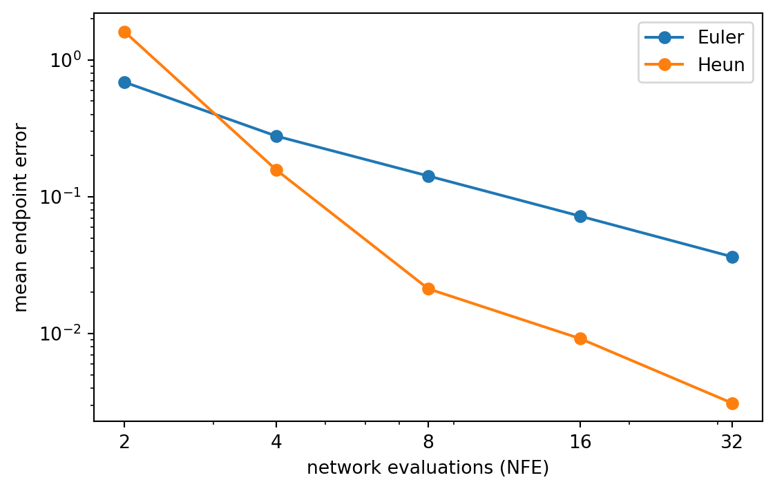
TL;DR — (NFE = number of function evaluations: how many times the denoiser is called.) A one-step update needs the interval-average velocity; an ordinary diffusion or flow model supplies only the instantaneous velocity at the current state. Solvers estimate that average from several evaluations. Straightening reduces the gap between instantaneous and interval-average velocity; in the constant-velocity limit they coincide. Finite-time maps predict the interval quantity directly. Distribution matching abandons the requirement that a given seed land anywhere in particular. Measured below: Heun is 2.3× worse than Euler at two network calls, and one round of reflow cuts the one-step energy-distance error by more than two orders of magnitude, while at 64 steps the remaining difference is below the seed-to-seed variation in this experiment.
Four ways to spend fewer evaluations
Before any mathematics, the map. These are mechanisms rather than mutually exclusive categories: real systems routinely combine them, and both InstaFlow and SDXL-Turbo use two.
What changes
Core idea
Representative work
Family 1 — integrate better
sampler only
estimate the same changing field more accurately
DPM-Solver++, UniPC, DEIS, EDM/Heun
Family 2 — make the field easier
trajectory / coupling
make typical paths straighter
Rectified Flow, reflow, InstaFlow
Family 3 — learn the finite jump
prediction target
predict an endpoint, a two-time map, or an interval average
Consistency Models, LCM, Shortcut, MeanFlow
Family 4 — match the destination
training objective
stop requiring seed-wise path reproduction
DMD/DMD2, ADD
Families 1–3 disagree about how to close the gap but agree on what counts as success: start from a particular noise sample and arrive where that sample should have arrived. The correspondence between seed and output is one-to-one, and preserving it is part of the goal.
Family 4 abandons that correspondence. It requires only that the population of generated samples match the target distribution. An individual seed may land somewhere other than where the teacher would have taken it, provided the ensemble comes out right. That is a strictly weaker requirement — every solution acceptable to Families 1–3 is also acceptable here, and many more besides — which is exactly what buys the extra freedom, and what produces the failure modes discussed at the end.
Setup — the two-blob toy from the previous post
Code
import timeimport torchimport torch.nn as nntorch.set_num_threads(4)torch.manual_seed(0)A, S =2.0, 0.35MU = torch.tensor([[-A, 0.0], [A, 0.0]])T_START, T_END =1.0, 1e-3def sample_data(n, g=None): which = torch.randint(0, 2, (n,), generator=g)return MU[which] + S * torch.randn(n, 2, generator=g)def denoiser(z, t):"""Exact E[x | z_t] for the two-blob data. Derived, not trained.""" t = torch.as_tensor(t, dtype=z.dtype) var_t = (1- t)**2* S**2+ t**2 sq = (z[:, None, :] - (1- t) * MU).square().sum(-1) w = torch.softmax(-0.5* sq / var_t, dim=1) prec =1/ S**2+ (1- t)**2/ t**2 m = (MU / S**2+ (1- t) * z[:, None, :] / t**2) / precreturn (w[..., None] * m).sum(1)def velocity(z, t):"""Direction of travel at (z, t): away from the noise, toward the signal.""" t = torch.as_tensor(t, dtype=z.dtype).clamp(min=1e-3) x_hat = denoiser(z, t)return (z - (1- t) * x_hat) / t - x_hat
Family 1 — integrate the same field better
The last post established that sampling is numerical integration of a learned field, so the first move is to integrate that same field more efficiently. In a real library this is exactly what the scheduler object does: diffusers exposes Euler, Heun, DEIS, DPM-Solver++ and UniPC as swappable schedulers for a compatible pretrained pipeline, and DPM-Solver was explicitly designed to produce good samples in roughly 10–20 evaluations.
Euler and Heun below are the two pedagogical representatives of that menu: diffusers exposes diffusion-specific versions as EulerDiscreteScheduler and HeunDiscreteScheduler, and Heun is the default second-order sampler in Karras et al.’s EDM. The three-line functions here are the bare integration rules, not those full implementations.
The stepping rule from last time is Euler’s method: look at the direction here, and go that way for the whole step.
def euler_step(z, t, t_next):"""Take the direction at the start of the interval and commit to it."""return z + (t_next - t) * velocity(z, t)
Its weakness is the one the last post identified: if the direction changes during the step, you followed a stale direction. The obvious repair is to check. Take the Euler step provisionally, look at the direction where you would land, and average the two. That is Heun’s method:
def heun_step(z, t, t_next):"""Look ahead with a provisional step, then average the two directions.""" h = t_next - t v_here = velocity(z, t) z_provisional = z + h * v_here # where Euler would have taken us v_there = velocity(z_provisional, t_next)return z + h *0.5* (v_here + v_there) # split the difference
Heun costs two network calls per step instead of one, which brings up the accounting rule that governs this whole subject:
Count network evaluations, not scheduler iterations. A 10-step Heun run uses 20 fresh field evaluations; 20 Euler steps use 20. Under the same model and batch shape, equal NFE is the right first comparison of denoiser work. It is still not a complete latency comparison.
The formal description of the difference is order: halve the step size and a first-order method’s error roughly halves, a second-order method’s falls by roughly four. Euler is first order, Heun is second.
def sample(z, n_steps, step_fn): ts = torch.linspace(T_START, T_END, n_steps +1)for i inrange(n_steps): z = step_fn(z, ts[i], ts[i +1])return zstart = torch.randn(6000, 2)reference = sample(start.clone(), 4000, heun_step) # so fine it's essentially exactdef error_at(nfe, step_fn, calls_per_step): result = sample(start.clone(), nfe // calls_per_step, step_fn)return (result - reference).norm(dim=-1).mean().item()print(f"{'NFE':>5}{'Euler':>10}{'Heun':>10} (equal network calls)")for nfe in [2, 4, 8, 16, 32]:print(f"{nfe:>5}{error_at(nfe, euler_step, 1):>10.4f} "f"{error_at(nfe, heun_step, 2):>10.4f}")
import matplotlib.pyplot as pltplt.rcParams.update({"font.size": 10, "axes.edgecolor": "#888888","axes.linewidth": 0.8, "xtick.color": "#666666","ytick.color": "#666666", "figure.dpi": 110})C_A, C_B ="#3B6EA5", "#B5561E"budgets = [2, 4, 8, 16, 32]euler_errors = [error_at(n, euler_step, 1) for n in budgets]heun_errors = [error_at(n, heun_step, 2) for n in budgets]fig, ax = plt.subplots(figsize=(6.2, 4))ax.loglog(budgets, euler_errors, "o-", color=C_A, lw=1.8, ms=7, mfc="white", mew=1.6, label="Euler (1st order)")ax.loglog(budgets, heun_errors, "o-", color=C_B, lw=1.8, ms=7, mfc="white", mew=1.6, label="Heun (2nd order)")ax.set_xscale("log", base=2)ax.set_xticks(budgets); ax.set_xticklabels(budgets)ax.set_xlabel("network evaluations (NFE)"); ax.set_ylabel("mean endpoint error")ax.grid(True, which="both", alpha=0.18); ax.legend(frameon=False, fontsize=9)for s in ax.spines.values(): s.set_alpha(0.5)ax.annotate("order inverts here", xy=(2, heun_errors[0]), xytext=(3.2, 1.9), fontsize=8.5, color=C_B, arrowprops=dict(arrowstyle="->", color=C_B, lw=1))plt.tight_layout(); plt.show()
Error at equal NFE. Higher order wins once the intervals are moderate, and loses in the extreme two-call regime.
e16, e32 = error_at(16, euler_step, 1), error_at(32, euler_step, 1)h16, h32 = error_at(16, heun_step, 2), error_at(32, heun_step, 2)print("what happens to the error when you double the budget:")print(f" Euler x{e32/e16:.2f} (first order predicts x0.50)")print(f" Heun x{h32/h16:.2f} (second order predicts x0.25)")
what happens to the error when you double the budget:
   Euler  x0.51   (first order predicts x0.50)
   Heun   x0.34   (second order predicts x0.25)
The theory holds and the practical consequence is large: at 32 network calls Heun’s error is roughly a tenth of Euler’s. A major early branch of diffusion acceleration — DEIS, DPM-Solver/DPM-Solver++, UniPC — reduced sampling cost this way, by changing the deterministic trajectory, its parameterisation, or its numerical integration without retraining the denoiser. DDIM belongs in this training-free branch historically and opened it, though it arrives from a different construction — a family of non-Markovian forward processes with a deterministic sampler as one member — rather than from higher-order integration of the same interval. These methods are training-free but not universally interchangeable: prediction type, noise schedule, timestep convention and preconditioning must match the checkpoint.
The caveat, at the extreme low end. Look again at the first row. At two network calls, Heun is more than twice as bad as Euler. Order is an asymptotic property — it describes what happens once steps are small enough for the local expansion behind the method to be informative. With one enormous Heun step the provisional point is already far off trajectory, near the singular low-noise endpoint, so averaging its derivative with the first makes the result worse. A correction step helps only when the point being corrected from is itself meaningful.
Order tells you an asymptotic rate, not who wins at one to four evaluations — which is exactly where few-step generation lives. Order is also not a cost model: Runge–Kutta methods spend extra evaluations per step, while multistep methods reuse ones they already made.
One equation behind the first three families
Before the remaining families, an identity that makes all of them obvious. Families 1–3 are all readable off this one equation; Family 4 will deliberately step outside it.
The displacement over an interval is the integral of the velocity along the path, which is by definition the interval length times the average velocity:
A one-step local update instead moves by \((s-t)\, v(z_t, t)\), using the direction at the start. Subtract them:
\[\text{one-step error} = |s-t| \cdot \lVert\, \underbrace{v(z_t, t)}_{\text{what the model gives you}} - \underbrace{\bar v_{t \to s}}_{\text{what you needed}} \,\rVert\]
Not a bound — an identity:
probe = torch.randn(3000, 2)reference_end = sample(probe.clone(), 800, heun_step) # fine numerical reference,# not an analytic endpointaverage_direction = (reference_end - probe) / (T_END - T_START) # displacement / timeinitial_direction = velocity(probe, torch.tensor(T_START))actual_error = (probe + (T_END - T_START) * initial_direction - reference_end).norm(dim=-1)predicted = ((T_END - T_START) * (initial_direction - average_direction)).norm(dim=-1)print(f"largest disagreement between the two, over 3000 samples: "f"{(actual_error - predicted).abs().max():.1e}")
largest disagreement between the two, over 3000 samples: 4.8e-07
Zero to floating-point precision. Which reorganises the whole problem — every remaining mechanism bridges the same gap differently:
Family 1 samples the local field several times and combines them, estimating \(\bar v\) better. Heun’s two evaluations are literally a two-point estimate of a mean. This also explains the floor: from one generic evaluation you cannot recover an interval average without extra assumptions about the field.
Family 2 attacks the other side. If the velocity remains constant along the path — same direction and same speed — then \(v(z_t,t) = \bar v\) exactly, the gap is zero, and one step is not approximately right but exactly right.
Family 3 sidesteps estimation by regressing the interval quantity — the endpoint, or \(\bar v\) itself — directly.
If the trajectory is affine in time its velocity is constant, so one Euler step integrates it exactly. That is a one-line consequence of \(z(t) = a + tb \Rightarrow v = b\), and needs no experiment. The interesting question is whether real learned trajectories can be made to look like that.
Family 2 — make the field easier to integrate
Rectified flow chooses linear conditional paths: \(z_t = (1-t)x + t\epsilon\) connects one data sample to one noise sample at constant conditional velocity \(\epsilon - x\). Every training path is perfectly straight. So why do the learned trajectories bend at all?
Because of which pairs get matched, and it is worth separating two families of curves that are easy to confuse.
Each training pair contributes one straight line, and the pairing is random, so many of those lines pass through the same point \((z, t)\) heading toward different destinations. The network cannot emit two directions at one input, and squared error makes it emit their average. This is the same averaging that made the denoiser return the dataset mean at \(t=1\), seen from the other side.
That average is a single well-defined field, and an ODE driven by a single-valued field has exactly one solution through each point. So the trajectories of the learned flow never cross, even though the training lines that produced it do.
The averaged field is correct: integrating it really does carry noise to data with the right distribution. But its trajectories are not the straight training lines. They are curves threading between them, and curvature is what costs evaluations.
So straightening is not about fixing an error. It is about finding a coupling whose averaged field bends less.
Reflow changes the pairing. Start from a noise sample \(\epsilon\), run the current model all the way to the data end, and call the endpoint \(T(\epsilon)\). Reflow then trains on
\[
(\epsilon,\;T(\epsilon))
\]
instead of pairing \(\epsilon\) with an independently drawn data sample.
Why should this make the field straighter?
With independent pairing, the endpoint assigned to a noise sample is arbitrary. Many training pairs can therefore pass through the same region while asking for different velocities, and squared-error training averages those targets. The resulting field is valid, but it can curve substantially.
Reflow uses a more coherent pairing: each noise sample is paired with the endpoint that the current flow already sends it to. The existing model may reach that endpoint along a curved trajectory; reflow now trains on the direct interpolation between the same start and end.
Across many such pairs, the regression problem becomes less ambiguous and the learned trajectories tend to straighten. The pairing preserves the start-to-end correspondence already realised by the current flow.
A finite reflow dataset is just a sample of this rule. Conceptually, the map \(T(\epsilon)\) exists for every noise input; using more sampled pairs only approximates that population training objective more accurately.
We can test that here, with an advantage a real system does not have: our underlying field is exact, so we generate the coupling with a fine numerical solve of the exact toy velocity field rather than with a learned teacher. The integration is still numerical — 200 Euler steps — so the coupling is a close approximation, not an analytic one. To keep the comparison fair, both fields below are networks with identical architecture, initialisation and training budget — the only difference is which pairs they see.
Code
class VNet(nn.Module):def__init__(self, h=128):super().__init__()self.f = nn.Sequential(nn.Linear(3, h), nn.SiLU(), nn.Linear(h, h), nn.SiLU(), nn.Linear(h, h), nn.SiLU(), nn.Linear(h, 2))def forward(self, z, t): t = torch.as_tensor(t, dtype=z.dtype).expand(z.shape[0]).view(-1, 1)returnself.f(torch.cat([z, t], 1))def train(pairs_fn, steps=4000, bs=1024, seed=0): torch.manual_seed(seed) net = VNet(); opt = torch.optim.Adam(net.parameters(), 2e-3)for _ inrange(steps): x, eps = pairs_fn(bs) t = torch.rand(bs, 1) zt = (1- t) * x + t * eps loss = ((net(zt, t.squeeze(1)) - (eps - x))**2).mean() opt.zero_grad(); loss.backward(); opt.step()return net@torch.no_grad()def integrate(vfn, z, n_steps, keep=False): ts = torch.linspace(T_START, T_END, n_steps +1) path = [z.clone()]for i inrange(n_steps): z = z + (ts[i+1] - ts[i]) * vfn(z, ts[i])if keep: path.append(z.clone())return (z, torch.stack(path), ts) if keep else z
independent =lambda n: (sample_data(n), torch.randn(n, 2))# reflow bank: couple each noise draw to the endpoint# from a fine numerical solve of the exact toy fieldtorch.manual_seed(1)z_bank = torch.randn(60_000, 2)x_bank = integrate(velocity, z_bank.clone(), 200)def reflow(n): i = torch.randint(0, z_bank.shape[0], (n,))return x_bank[i], z_bank[i]t0 = time.time()net_base = train(independent, seed=0)net_rf = train(reflow, seed=0) # same init, same arch, same budgetprint(f"[trained both fields in {time.time() - t0:.0f}s on CPU]")
[trained both fields in 36s on CPU]
One check is required before any of this can be interpreted. The reflow bank is generated rather than drawn from the data, so the second model is fitting a slightly different target distribution. How different?
The comparison below uses energy distance: a distance between two distributions computed only from average pairwise distances between samples. It is small when the two sets are thoroughly interleaved, large when they sit apart, and zero exactly when the distributions match. It is used here because it needs only samples, not densities — and because, being a single number summarising a whole distribution, it must always be read against the scale set by two draws of real data.
def energy(a, b): d =lambda p, q: torch.cdist(p, q).mean()return (2* d(a, b) - d(a, a) - d(b, b)).item()real = sample_data(4000, torch.Generator().manual_seed(8))# real-vs-real is itself a finite-sample quantity, so measure its spreadbaseline = [energy(sample_data(4000, torch.Generator().manual_seed(s)), sample_data(4000, torch.Generator().manual_seed(s +50)))for s in [8, 9, 10, 11, 12]]print(f"real-vs-real over 5 seed pairs : {min(baseline):.4f} to {max(baseline):.4f}")print(f"energy(reflow bank, real) = {energy(x_bank[:4000], real):.4f}")
real-vs-real over 5 seed pairs : 0.0002 to 0.0009
energy(reflow bank, real)      = 0.0009
The bank sits at the upper edge of the range two independent draws of real data produce at this sample size — comparable in magnitude to sampling variation, but marginally above it rather than demonstrably inside it. So the coupling is close to, but not identical to, the data distribution. With a learned teacher the gap can be considerably wider, because teacher error is inherited by the generated pair bank; here the intervention is close to coupling-only.
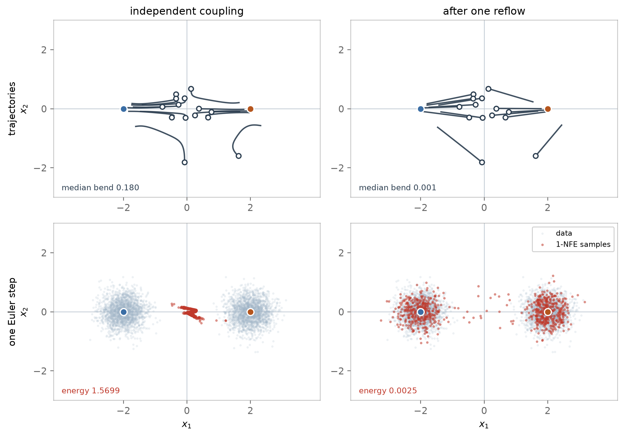
Now measure straightness, using the bend metric from the previous post. In words: take the straight line joining a trajectory’s own start and end, find the point where the trajectory bows furthest away from that line, and divide that distance by the length of the line. Zero means the path is exactly straight; 0.2 means it wanders about a fifth of the endpoint distance off the direct route. Dividing by the chord length makes it scale-free, so paths of different lengths are comparable.
median bend, exact field        : 0.178
median bend, trained (independent): 0.180
median bend, trained (reflowed)   : 0.001
Two things there. The independently-coupled network reproduces the exact field’s bend closely, which confirms it learned the field rather than something else. And reflow removes essentially all of the curvature.
Same architecture, same budget, same starting noise — only the coupling differs. Top: trajectories. Bottom: where a single Euler step lands. The base model’s one step collapses toward the mean between the modes; the reflowed model’s recovers both blobs.
print(f"{'NFE':>5}{'base':>12}{'reflowed':>12}{'ratio':>9}")ratios = {}for nfe in [1, 2, 4, 8, 16, 64]: ea = energy(integrate(net_base, z_test.clone(), nfe), real) eb = energy(integrate(net_rf, z_test.clone(), nfe), real) ratios[nfe] = ea / ebprint(f"{nfe:>5}{ea:>12.4f}{eb:>12.4f}{ea/eb:>8.1f}x")# the prose above claims "more than two orders of magnitude" at one step, and# that the advantage decays with NFE. Assert both, so a re-render on different# hardware cannot leave the text behind.assert ratios[1] >100, f"one-step ratio {ratios[1]:.0f} no longer supports the claim"assert ratios[64] < ratios[1] /50, "the advantage should decay with NFE"
Read the two ends separately. At one step the difference is enormous. The base model’s single Euler step extrapolates the \(t=1\) velocity across the whole interval, which is valid only if that velocity holds throughout — and it does not. The reflowed model’s single step is nearly as good as its sixty-four.
At sixty-four steps the gap has closed. Whether it has closed exactly is not something one run can answer, so repeat the pipeline across three seeds:
Code
def run_seed(s, steps=1500, bs=512): nb = train(independent, steps=steps, bs=bs, seed=s) torch.manual_seed(100+ s) zb = torch.randn(20_000, 2); xb = integrate(velocity, zb.clone(), 200) pf =lambda n: (lambda i: (xb[i], zb[i]))(torch.randint(0, 20_000, (n,))) nr = train(pf, steps=steps, bs=bs, seed=s) e =lambda net, k: energy(integrate(net, z_test.clone(), k), real)return e(nb, 1), e(nr, 1), e(nb, 64), e(nr, 64)rows = [run_seed(s) for s in [0, 1, 2]]print(f"{'seed':>5}{'base N=1':>11}{'reflow N=1':>13}{'base N=64':>12}{'reflow N=64':>14}")for s, r inzip([0, 1, 2], rows):print(f"{s:>5}{r[0]:>11.4f}{r[1]:>13.4f}{r[2]:>12.4f}{r[3]:>14.4f}")b64 = [r[2] for r in rows]; r64 = [r[3] for r in rows]print(f"\nN=64 spread: base {max(b64)-min(b64):.4f} reflow {max(r64)-min(r64):.4f}")print(f"N=64 |mean difference| {abs(sum(b64)/3-sum(r64)/3):.4f}")
These runs use a smaller budget than the headline pair, so the absolute numbers sit higher; what matters is the comparison within each row. The one-step advantage is large and consistent at every seed. At sixty-four steps the mean difference between the two models is smaller than the base model’s own run-to-run spread, so this experiment cannot separate them — not that they are provably equal.
Reflow requires generating a large synthetic dataset with the teacher, and each round inherits whatever the teacher got wrong. In practice it is also rarely used alone — InstaFlow’s released one-step model combines rectification with subsequent distillation.
Family 3 — learn finite-time transport
The distinction from Family 2 is important.
Family 2 keeps the model local. It still predicts an instantaneous velocity \(v(z_t,t)\), but changes the training geometry so that this local velocity remains useful over a larger interval. The goal is to make the trajectory easier to integrate.
Family 3 changes the prediction target. The trajectory may remain curved. Instead of approximating a long move by repeatedly querying a local velocity, the model is trained to predict a finite-time quantity directly — an endpoint, a future state, or an interval-average velocity.
So the two strategies solve the same problem in opposite ways:
\[
\boxed{
\begin{aligned}
\text{Family 2:}&\quad \text{make the path easier for a local model to follow},\\
\text{Family 3:}&\quad \text{teach the model to jump farther along the path directly}.
\end{aligned}
}
\]
Train a model whose output already describes a finite interval. The organising question is: what finite object should the model predict? There are three useful answers.
Endpoint maps: consistency models
For an endpoint consistency model,
\[
f(z_t,t)\approx z_0.
\]
The important point is that \(f\) is not another velocity field. It does not say which infinitesimal direction to move next. It asks a finite-time question:
given this state on the trajectory, where does this trajectory eventually end?
Training therefore encourages states sampled at different times along the same ODE trajectory to agree on the same endpoint.
The curvature of that trajectory is irrelevant to the definition. A highly curved trajectory can still have a perfectly well-defined endpoint. Family 2 tries to reduce that curvature so numerical integration becomes cheap; consistency models instead learn the endpoint map directly.
Any two points on the same probability-flow trajectory must decode to the same endpoint, so the defining requirement is self-consistency along a trajectory, together with a boundary condition \(f(z_\varepsilon, \varepsilon) = z_\varepsilon\) that pins down which endpoint. Two routes lead there, and they differ in what supplies the second point.
Consistency distillation takes it from a pretrained diffusion model: run the teacher’s solver one small step from \(z_t\), then require the student to decode the original and the stepped point identically. The teacher supplies a reliable trajectory, which makes the target well behaved and the optimisation comparatively stable. The costs are that someone must train the teacher first, and that the student inherits both its quality ceiling and its systematic errors. This is the route behind the models people actually deploy — Latent Consistency Models and LCM-LoRA.
Consistency training removes the teacher and estimates the same adjacent-state relation directly from data and the known interpolant. Nothing caps the student at teacher quality, but the estimate is noisier, and the method was historically sensitive to discretisation and schedule choices; later continuous-time formulations removed much of that tuning burden.
In neither case is a teacher-provided clean endpoint the regression target. What is being matched is the agreement between two points on one trajectory.
Does crossing cause trouble here? The answer becomes clear once we separate different kinds of curves.
1. Pairwise training paths.
In flow matching, a chosen pair \((x,\epsilon)\) defines the straight interpolation
\[
z_t = (1-t)x + t\epsilon.
\]
These are artificial paths used to construct training targets. With independent pairing, different paths can pass through the same region at the same time while prescribing different velocities. The regression then averages those targets — the Family 2 effect.
2. Learned ODE trajectories.
After training, the network defines one velocity \(v(z,t)\) at each state and time:
\[
\frac{dz}{dt} = v(z,t).
\]
Under the usual uniqueness conditions for an ODE, a particular state-time pair \((z_t,t)\) has one continuation. It therefore has one endpoint. This is the path that matters for consistency models.
So self-consistency is asking for something well defined:
different states sampled along the same ODE trajectory should predict the same endpoint.
There are no conflicting endpoint targets at the same \((z,t)\) to average.
So the distinction is:
Family 2 changes the coupling used to learn the velocity field; Family 3 learns finite-time maps along the ODE trajectories defined by that field.
Family 3 has a different difficulty: near pure noise, nearby states can still end at very different clean samples, so the endpoint map can vary sharply even though it remains single-valued.
Two-time maps: trajectories, shortcuts, flow maps
An endpoint map answers only “where does this finish?”. Generalise by giving the model a destination time:
\[f(z_t, t, s) \approx z_s\]
Now one network can make a long jump or several short ones, and maps compose when a larger budget is available. Consistency trajectory models learn transitions to arbitrary later points; shortcut models condition explicitly on the requested step size, so one set of weights serves both local and long updates; flow-map models treat the two-time transition as the central object. The advantage is adjustable compute: the model is trained for the kind of finite jump it will actually make, instead of hoping a local derivative stays valid.
Interval-average velocity: MeanFlow
The third answer connects back to the identity exactly. We said the sampler needs \(\bar v\). So predict \(\bar v\).
As written, this is useless as a training target. The right-hand side is an integral along a trajectory we would have to simulate, which is precisely the cost we are trying to avoid. The goal is to turn this definition into a relation between quantities we already have, and the standard move for making an integral local is to differentiate it.
Differentiate both sides with respect to \(t\), holding \(r\) fixed.
The left side is a product of \((t-r)\) and \(u\), so it gives \(u + (t-r)\frac{du}{dt}\).
The right side gives \(v(z_t, t)\), by the fundamental theorem of calculus: differentiating an integral with respect to its upper limit returns the integrand evaluated at that limit.
Read it in words: the interval average is the instantaneous velocity, minus a correction for how much the velocity changes across the interval. As \(r \to t\) the interval closes, the correction term vanishes, and \(u = v\) — the average over an infinitesimal interval is the instantaneous value, as it has to be. The longer the interval, the more work the correction does.
What are we differentiating if \(u\) is the thing we are trying to learn?
We do not know the true interval-average field \(u\). We represent it with a neural network
\[
u_\theta(z,r,t).
\]
During training, that network already gives a current estimate of \(u\). Because \(u_\theta\) is differentiable, automatic differentiation can also tell us how the current prediction changes when its inputs change. MeanFlow uses that derivative to construct the target that improves \(u_\theta\).
So we are not differentiating an unknown oracle. We are differentiating the current network.
The total derivative. Hold \(r\) fixed and advance time by a tiny amount \(dt\). Two inputs change together:
\[
t \rightarrow t + dt,
\]
and, because the state follows the flow,
\[
z_t \rightarrow z_t + v\,dt.
\]
The prediction therefore changes because time moved and because the state moved. The chain rule gives
The \(3\) comes from advancing time; \(2zv\) comes from moving the input \(z\).
What is the Jacobian? For a vector-valued network, \(\nabla_z u_\theta\) is a matrix of sensitivities: entry \((i,j)\) says how output component \(i\) changes when input component \(j\) changes.
MeanFlow never needs that whole matrix. It only needs
\[
(\nabla_z u_\theta)v,
\]
the change in the output when the input is nudged specifically in direction \(v\). Equivalently,
That is a Jacobian-vector product (JVP): a directional derivative, not an explicitly constructed Jacobian.
For MeanFlow, \(z\) moves with velocity \(v\), \(t\) advances at rate \(1\), and \(r\) stays fixed.
Everything on the right-hand side is now available during training: \(v\) is the ordinary flow-matching target, and the correction is one JVP through the network being trained. The target is detached and the model regresses onto it. So the average-velocity model can be trained without a teacher, without distillation, and without a curriculum.
Generation is one line. Once \(u\) is learned, rearrange the definition:
\[z_r = z_t - (t-r)\,u(z_t, r, t)\]
No JVP appears here. It is a training-time mechanism for constructing the target, not a solver invoked at generation time. One network call moves you a finite distance.
Why this removes integration error. That update is the definition of \(u\) rearranged, not an approximation of it. Nothing was truncated, so there is no discarded Taylor remainder: if \(u\) were exact, the finite jump would be exact too, however long the interval. Contrast Euler, where even a perfect \(v\) leaves an \(O(h^2)\) remainder at every step. The error has not vanished — it has changed category, from integration error, which you can shrink by taking more steps, to approximation error in how well the network learned \(u\), which you cannot. MeanFlow reported 3.43 FID at one NFE on ImageNet \(256^2\) trained from scratch, and the direct-training frontier has since broadened — Improved MeanFlow, and Pixel MeanFlow which moves the objective to latent-free pixel generation. Those paper-reported numbers are not clean rankings: architectures, compute, data processing and evaluation protocols all differ.
Family 4 — match the destination distribution
Families 1–3 retain a particular finite-time transport problem tied to the starting state. Family 4 drops the seed-wise correspondence and constrains the output population instead.
Pointwise: same seed → approximately the teacher’s corresponding sample. Distribution matching: many generated samples → the correct population.
Distribution matching distillation (DMD, DMD2) trains a few-step generator so its output distribution approaches the target, represented by real data and/or a pretrained teacher. The distribution-matching objective itself does not require the student to land where the teacher would for a given seed, though real systems often combine it with other losses. Adversarial distillation (ADD, LADD) adds a discriminator to the same goal and produced the SDXL-Turbo line, which runs in a single step and is supported natively in diffusers.
The distinction predicts the failure modes:
Pointwise teacher-following anchors the student to the teacher’s noise-to-image mapping. That preserves behaviour, and also transfers systematic weaknesses unless something counteracts them.
Distribution-level objectives constrain only the population. They can improve on teacher weaknesses, but the weaker anchoring makes diversity drift and prompt-specific regressions easier to hide behind a healthy aggregate score.
That second point is not hypothetical: 1.x-Distill’s stated motivation is precisely that DMD suffers diversity collapse when pushed to two steps or fewer.
Conditional generation is where the boundary bites hardest. In text-to-image the requirement really is distributional: many different images are acceptable for one prompt, so an objective constraining the population is well matched to the task. Restoration and other inverse problems are not like that. The output is judged against this input, and “plausible, but not faithful to the degraded image” is a failure rather than a variation. A purely distributional objective does not penalise it, because population statistics can look healthy while individual reconstructions drift away from their inputs. This follows from what the objective does and does not constrain rather than from anything measured here; in practice, conditional few-step systems tend to combine a distributional term with a fidelity or regression term rather than relying on the former alone.
The four families, side by side
Retrains?
Typical NFE
What it costs you
What it risks
1 Solvers
no
~10–25
nothing; must match the checkpoint
hits a model-dependent floor; higher order can lose at extreme low NFE
2 Reflow / straightening
usually
model-dependent
reflow needs generated pairs + a retraining round
pairing and teacher bias; straightness is not guaranteed
3 Finite-time maps
yes
1–4
distillation or from-scratch training
approximation error replaces integration error
4 Distribution matching
yes
1–4
training + auxiliary networks
diversity collapse under a healthy aggregate metric
If you have a pretrained model and want it faster this week, the ordering is: exhaust the free options first (compatible solver, tuned step placement), measure where the time actually goes, and only then consider training something.
What to carry away
Count NFE, not steps. Heun at 10 steps costs 20 fresh calls. Equal NFE is the fair first comparison of denoiser work; wall-clock latency still needs measuring.
Order is asymptotic and can invert. Heun is 2.3× worse than Euler at two network calls, because its look-ahead lands somewhere meaningless. Formal order is also not a cost model.
The exact requirement: one-step error is the gap between the instantaneous direction the model gives you and the interval-average direction you need. Solvers estimate the average; straightening makes them equal; MeanFlow models the average directly.
The coupling curves the flow, not the interpolant. Every training path was straight; the learned field still bent by 0.18 of the chord, and changing only which pairs were matched took that to 0.001.
Reflow’s measured benefit sat at low NFE. One-step energy-distance error fell by more than two orders of magnitude; at 64 steps the difference was smaller than the base model’s own seed-to-seed spread, so this experiment could not separate them.
Family 4 changes the question. Constraining the output population rather than the seed-wise mapping is a different commitment, with different failure modes — chiefly diversity collapse that aggregate metrics do not show.
If one sentence survives: local models predict what to do now; fast generators either estimate, simplify, or directly learn what should happen over a finite interval.
Where this goes next
Four mechanisms, derived from one finite-time problem; the first two measured on a two-dimensional toy where the underlying field is known exactly. That is enough to see the mechanisms and not enough to say anything about images. The next post trains representative versions of these on real image data, runs the released models people actually deploy, and measures what each one costs in latency rather than in evaluations.