A diffusion model runs the same network dozens of times to make one picture. This post asks why it cannot run it once — and answers with an experiment where the network is provably perfect and the sampler still fails completely.
generative
diffusion
Published
August 1, 2026
Generate an image with a diffusion model and watch what the GPU does. It runs the same network, with the same weights, twenty to fifty times. Each run nudges the current picture. Only after the last one do you get an image.
That should feel wasteful. One network, one prompt — why fifty passes for one answer?
The tempting explanation is that the network isn’t good enough, and a better one would need fewer passes. That explanation is incomplete. Below we build a case where the model is provably exact and a single-pass sampler still fails completely. The experiment isolates a second error source that is easy to miss: a correct local prediction can be used in a bad long-range update.
TL;DR — The network answers a question about the state you have right now. The sampler must turn a sequence of those local answers into a complete trip from noise to image. At pure noise the correct answer is the dataset mean, so one giant step lands there even with a perfect model. Re-evaluating as the state changes lets the answer become mode-specific, then instance-specific. Sampling cost is the price of tracking a field that changes underneath you — and with a first-order sampler that error falls as \(1/n\) in the number of steps, which we measure.
Why corrupt data and then reverse it?
Generation means drawing new samples from a distribution we only have examples of. Done directly that is hard — the density is unknown and high-dimensional.
Noise makes it easy in one specific sense: add enough Gaussian noise to any distribution and what remains is almost exactly a standard Gaussian, which we can sample trivially. That gives a bridge. Forward, corruption connects the data to a distribution we can sample from. Reverse, walking that bridge backwards from pure noise produces a fresh sample.
The reason this is learnable is that it never asks for the hard thing. Learning to map noise straight to data in one shot is a difficult regression. Learning to undo a small amount of corruption is much easier, and the bridge lets us chain those easy problems together instead of solving the hard one.
The network answers a question about a single state: given this noisy sample at this noise level, what does the clean data behind it look like. The sampler is the numerical procedure that turns a sequence of those answers into a complete path from noise to image — it decides where to evaluate, how far to move, and how to combine what it gets back. The network supplies directions; the sampler does the travelling. Neither generates anything alone.
The asymmetry between the two directions is the subject. Forward needs no iteration at all: any noise level is one closed-form draw from a clean sample. Reverse cannot be shortcut that way, because it follows a learned field and has to integrate it.
A distinction worth making early, because two different arguments both end at “many steps” and they are easy to conflate. In the original stochastic formulation, the reverse transition is only approximately Gaussian when the interval is short, which is what motivated a long chain in the first place (Sohl-Dickstein et al., 2015; Ho et al., 2020). This post is about a second, separate reason: even with a deterministic sampler and an exact model, integrating a curved field in too few jumps is inaccurate. The experiment below isolates that second effect, which is why it uses a deterministic path and a denoiser that cannot be wrong.
What the network actually computes
Diffusion and flow models use several noise parameterisations. To isolate the sampling problem we use the linear path
\[z_t = (1-t)\,x + t\,\epsilon, \qquad t \in [0,1] \tag{1}\]
with \(x\) a clean sample and \(\epsilon \sim \mathcal{N}(0, I)\). At \(t=0\) the state is data; at \(t=1\) it is pure noise. Models may predict \(\epsilon\), \(x\), a score, or a velocity; away from the endpoints these are algebraically interchangeable given the schedule. We use the clean-sample form and call it a denoiser.
Now the subtlety that turns out to be the whole story. Many clean samples could have produced the same noisy \(z_t\) — that is what noise does. The network is trained under squared error, so it does not pick one plausible clean sample. Its optimum is the conditional average:
\[D(z_t, t) = \mathbb{E}[x \mid z_t] \tag{2}\]
Squared-error training does not merely drift toward the average; the average is its exact optimum. A perfectly trained denoiser returns it by construction.
Squared error is also not an arbitrary choice. The variational bound in the original derivation reduces, after reparameterisation, to a weighted squared-error regression, which is why essentially every diffusion model is trained this way (Ho et al., 2020).
The output is an average, and how much it averages over depends on the noise level. Read that in terms of the set being averaged. At high noise, corruption has destroyed most of what distinguished the original sample, so a wide and varied range of clean samples remain plausible explanations of \(z_t\) — and the average of a wide, varied set resembles nothing in particular. At low noise little has been destroyed, only a narrow band of samples is consistent with what you see, and their average is close to any one of them. The rule never changes: the output is always an average. What changes is how much it is averaging over.
One word to fix now, because several later arguments depend on it. The denoiser’s prediction is local: it holds at this state and this noise level, with no guarantee it stays valid once you move away from either. A sampler that treats it as valid over a long stretch of the journey is making an assumption the network never made.
Locality is a modelling choice, not a law of nature. The network is a function of \((z_t, t)\) and nothing else — it never sees where the trajectory came from or where it is heading, so it cannot return an answer that depends on either. Condition the network on more, or ask it for a different object entirely, and the locality changes. That is precisely what the fast-sampling methods in the next post do.
A toy where the model cannot be wrong
On a real model a bad one-step image has two suspects — the network guessed wrong, or the sampler misused a correct guess — and no way to separate them.
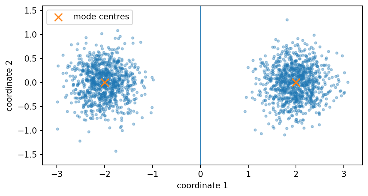
So we use data simple enough that the exact denoiser is a formula. Any failure is then unambiguously the sampler’s. Our dataset is two Gaussian blobs at \((\pm 2, 0)\).
Code
import torchimport matplotlib.pyplot as plttorch.manual_seed(0)plt.rcParams.update({ # a light, consistent look for every figure"font.size": 10, "axes.edgecolor": "#888888", "axes.linewidth": 0.8,"xtick.color": "#666666", "ytick.color": "#666666", "figure.dpi": 110,})A =2.0# distance of each blob from the originS =0.35# blob standard deviationMU = torch.tensor([[-A, 0.0], [A, 0.0]]) # the two centresC_LEFT, C_RIGHT ="#3B6EA5", "#B5561E"# the two modes, reused in every figureC_PATH, C_STEP, C_DATA, C_GRID ="#2C3E50", "#C0392B", "#9FB4C7", "#B9C4CE"def sample_data(n): which = torch.randint(0, 2, (n,))return MU[which] + S * torch.randn(n, 2)def _frame(ax): # shared coordinate frame for the 2-D plots ax.set_xticks([-2, 0, 2]); ax.set_yticks([-1, 0, 1]) ax.axhline(0, color=C_GRID, lw=0.7, zorder=0) ax.axvline(0, color=C_GRID, lw=0.7, zorder=0)for s in ax.spines.values(): s.set_alpha(0.5) ax.set_xlabel("$x_1$")def _modes(ax): # the two centres, drawn identically everywherefor mu, c inzip(MU, (C_LEFT, C_RIGHT)): ax.scatter(*mu.tolist(), marker="o", s=55, c=c, edgecolors="white", linewidths=1.3, zorder=6)
The dataset: two Gaussian blobs at (±2, 0), standard deviation 0.35.
Two blobs is the smallest dataset with a real generative choice: left mode or right mode. That is the one property of real images we need — a photo is of a dog or a cat, not a blend, and the central difficulty in generation is committing to one. It is deliberately not a stand-in for anything else about images. Two dimensions rather than one, because a curve in 1-D is a straight line by definition and we are going to measure curvature.
Deriving the exact denoiser
We want \(\mathbb{E}[x \mid z_t]\) in closed form. Two facts make that possible.
First, the forward path keeps Gaussians Gaussian. If \(x \sim \mathcal{N}(\mu_k, S^2 I)\) then \(z_t = (1-t)x + t\epsilon\) is a sum of two independent Gaussians — \((1-t)x\) with mean \((1-t)\mu_k\) and variance \((1-t)^2 S^2\), and \(t\epsilon\) with mean \(0\) and variance \(t^2\) — and independent Gaussians add in both, giving
The centre shrinks toward the origin and the spread grows. So the noisy distribution is a mixture of two known Gaussians — no approximation anywhere.
Second, the question splits in two:which blob did this come from? and given that blob, where in it?
For the first, each blob’s likelihood of \(z_t\) is the Gaussian of Eq. (3); the two priors are equal and cancel, so Bayes’ rule leaves a posterior that depends only on squared distance to each shifted centre, and normalising the two exponentials is exactly a softmax:
The temperature \(\sigma_t^2\) sets the softness: at high noise the two blobs overlap and the weights sit near \(\tfrac12\); as noise falls the nearer centre wins sharply. (These are the standard responsibilities of a Gaussian mixture — Bishop, PRML §2.3.9.)
For the second, a Gaussian prior with a Gaussian likelihood has a Gaussian posterior whose mean is a precision-weighted blend of the prior centre and the rescaled observation — each pulled in proportion to how certain it is (the conjugate Gaussian posterior — Bishop, PRML §2.3.3):
At small \(t\) the observation term dominates and \(m_k\) tracks \(z_t\); at large \(t\) the prior dominates and \(m_k\) collapses onto \(\mu_k\). Combining:
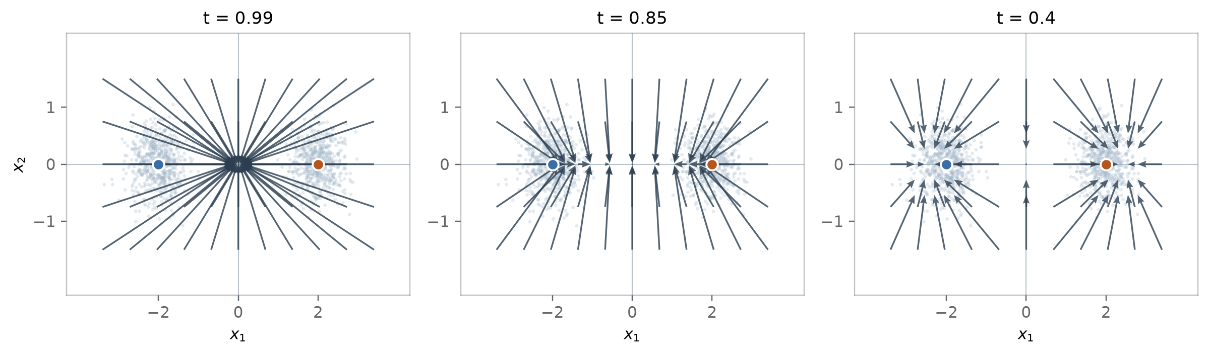
The denoiser’s answer sharpens as noise falls. At t=0.99 every input maps to essentially one point, the dataset mean. At t=0.85 the answers split in two. At t=0.4 they are specific to the input. Faint points show the data.
Three regimes, worth naming because the rest of the post uses the terms:
noise level
the denoiser’s answer is
called
\(t \to 1\)
the mean of the whole dataset
global
middling \(t\)
the centre of one blob
mode-specific
\(t \to 0\)
this particular point
instance-specific
That changing specificity is the mechanism behind everything below.
Trajectories and the velocity field
To sample we must move, so we need a direction. Differentiate the path (1):
\[\frac{dz_t}{dt} = \epsilon - x \tag{7}\]
That is the velocity: the rate at which a state moves as noise increases. Sampling runs the other way, so we follow \(-dz_t/dt\). In code we keep this forward velocity and integrate with a decreasing\(t\); the negative time increments supply the reversal, which is equivalent to following \(-v\) forward in time.
We do not know the particular \(x\) and \(\epsilon\) behind a given state — that is exactly what the noise destroyed. So we substitute their conditional averages: \(\hat{x} = D(z_t,t)\) from Eq. (6), and the noise implied by the path, \(\hat{\epsilon} = (z_t - (1-t)\hat{x})/t\).
T_START, T_END =1.0, 1e-3def velocity(z, t):"""Eq. (7) with conditional means substituted for the unknown x and ε.""" t = torch.as_tensor(t, dtype=z.dtype).clamp(min=1e-3) x_hat = denoiser(z, t) eps_hat = (z - (1- t) * x_hat) / treturn eps_hat - x_hat
Attach that arrow to every point in space and you have a velocity field. A trajectory is the path traced by following it: forward, a clean sample dissolving into noise; reverse, a noise sample resolving into data. Generation walks a reverse trajectory.
The field is local in both arguments — it depends on where you are and on the current noise level. Two consequences, and both are why one evaluation cannot suffice: the arrow at your current position tells you nothing about the arrow further along, and the whole field is different at every \(t\).
Why should the field change at all? Because the arrow is assembled from the denoiser, and the denoiser’s answer changes character as noise falls — exactly the three regimes above. Early it points at the dataset mean; later at the centre of one blob; at the end at a specific point. Those are different directions, so a trajectory that follows them has to turn. Curvature is the default rather than a pathology: a field pointing the same way throughout would mean the denoiser had learned nothing between \(t=1\) and \(t=0\). How curved, and whether it can be made straighter, is the subject of the next post.
Could one evaluation ever be enough?
Nothing above says a single evaluation is impossible in principle. Following the field from \(t=1\) down to \(t=0\) defines a deterministic map from a noise sample to a data sample — the flow map — and that map is a perfectly well-defined function. If a network could output it directly, generation would take one call.
The obstacle is that the local denoiser does not hand it to you. \(\mathbb{E}[x \mid z_t]\) answers a question about the state you currently hold; the flow map answers a question about an entire trajectory, and no algebra converts the first into the second without integrating. Learning the flow map directly is possible, but it is a different and harder regression problem, because the target is the outcome of a whole journey rather than a property of a single point. Much of the next post is about methods that attempt exactly that.
Euler steps, and why more of them help
For a general learned field whose trajectory is not available in closed form, we approximate the continuous evolution using a finite number of field evaluations. The Euler step is the simplest: read the velocity where you are, assume it holds for the whole interval, move.
\[z_{t+h} = z_t + h \cdot v(z_t, t) \tag{8}\]
That is precisely the first two terms of a Taylor expansion. Expanding the exact solution around \(t\):
Euler keeps the first two terms and discards the remainder. The assumption that the velocity holds for the whole interval is not an informal description of the method — it is the truncation, and it is false whenever the velocity changes along the interval. The resulting error is discretisation error, the cost of replacing a curve with finitely many straight jumps. It has nothing to do with the model being wrong.
Why more steps help, in two moves.
One step. The error a single step makes is the discarded remainder, roughly \(\tfrac{1}{2}h^2 \lvert z'' \rvert\). It is quadratic in \(h\): halve the step and each individual mistake becomes about four times smaller. The second derivative \(z''\) is how fast the velocity is changing, so a field that turns sharply costs more per step — which is why the bending we measure later is the quantity that matters.
The whole trip. Covering a fixed interval takes \(n \approx T/h\) steps. If the per-step errors simply added up, the total would be
One power of \(h\) survives, not two. Halving the step quarters every mistake but doubles how many you make, and quartering twice as often nets a halving. Since \(h\) is proportional to \(1/n\), the total error scales as \(O(h) = O(1/n)\) — Euler’s first-order convergence, and the reason a doubling of the step count buys a halving of the error rather than a quartering.
(The errors do not literally add. Each one is carried forward and stretched or damped by the remaining flow, so the rigorous statement carries a stability factor depending on how strongly the field varies. That factor changes the constant, not the power of \(h\).)
The plot below measures this rate.
def sample(z, n_steps):"""Walk from t=1 to t≈0 in n_steps equal Euler moves — Eq. (8).""" ts = torch.linspace(T_START, T_END, n_steps +1)for i inrange(n_steps): z = z + (ts[i +1] - ts[i]) * velocity(z, ts[i])return z
Code
torch.manual_seed(0)start = torch.randn(3000, 2)reference = sample(start.clone(), 8000) # fine enough to count as exactns = [1, 2, 4, 8, 16, 32, 64, 128]errs = [(sample(start.clone(), n) - reference).norm(dim=-1).mean().item() for n in ns]fig, ax = plt.subplots(figsize=(6.2, 4.0))C = errs[-1] * ns[-1] # anchor the 1/n guide at the finest runax.plot(ns, [C / n for n in ns], "--", color="#999999", lw=1.4, label="slope $-1$ (ideal $1/n$)", zorder=1)ax.plot(ns, errs, "o-", color=C_PATH, lw=1.8, ms=7, mfc="white", mew=1.6, label="measured", zorder=3)ax.set_xscale("log", base=2); ax.set_yscale("log")ax.set_xticks(ns); ax.set_xticklabels(ns)ax.set_xlabel("number of Euler steps $n$"); ax.set_ylabel("mean distance from reference")ax.grid(True, which="both", alpha=0.18); ax.legend(frameon=False, fontsize=9)for s in ax.spines.values(): s.set_alpha(0.5)ax.annotate("one step:\nlands on the mean", xy=(1, errs[0]), xytext=(2.1, 1.15), fontsize=8.5, color=C_STEP, ha="left", arrowprops=dict(arrowstyle="->", color=C_STEP, lw=1))plt.tight_layout(); plt.show()
Endpoint error against step count, log–log. From about eight steps the measured error lies on the dashed slope −1 line: each doubling halves it, Euler’s O(1/n) rate. At very coarse steps it sits above the line, outside the asymptotic regime, and one step is a catastrophe of its own.
From about eight steps on, each doubling of \(n\) halves the error — the straight, slope \(-1\) stretch of the plot, consistent with the \(O(1/n)\) rate above. The first couple of doublings beat that factor of two, and the measured curve sits above the \(1/n\) line there: at very coarse steps the error has not reached its asymptotic form, and a single step is a special catastrophe. This is the honest answer to “why fifty”: each doubling buys a halving, so you stop once the residual falls below what you can see. Fifty is not a fundamental constant — it is set by how fast the field turns, the order of the sampler, the noise schedule, and how much error you are willing to tolerate.
The one-step catastrophe
Now the extreme case: a single Euler step across the entire journey, with an exact denoiser, against a well-resolved run.
If the model were the only thing that mattered, one step should give a blurry but recognisable version of the data — points somewhere near each blob. Watch instead.
careful = sample(start.clone(), 4000)single = sample(start.clone(), 1)def near_a_blob(x):"""Fraction within 3σ of either centre. In 2-D the radial distance is Rayleigh, so the ceiling is 1 − exp(−9/2) ≈ 98.9%, not the 1-D 99.7%."""return ((x[:, None, :] - MU).norm(dim=-1).min(1).values <3* S).float().mean()print(f"{'sampler':>12}{'near a blob':>14}{'spread':>10}{'mean position':>20}")for name, out in [("4000 steps", careful), ("1 step", single)]:print(f"{name:>12}{near_a_blob(out):>13.1%}{out.std(0).max():>10.4f}"f"{f'({out[:,0].mean():+.3f}, {out[:,1].mean():+.3f})':>20}")
     sampler   near a blob    spread       mean position
  4000 steps        98.7%    2.0173    (-0.082, -0.001)
      1 step         0.0%    0.0010    (-0.000, -0.000)
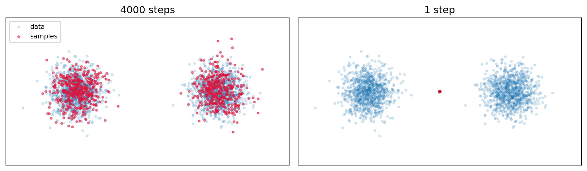
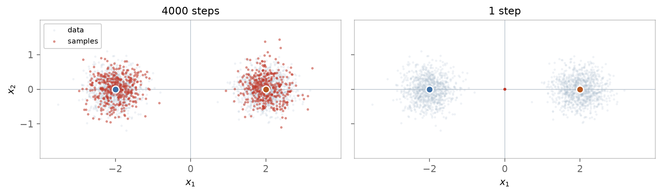
Left: 4000 steps recovers both modes. Right: one step puts every sample on the origin — a location the data never occupies.
Not degraded — annihilated. Every sample landed on essentially the same point, the average of the two blobs, a location the data never occupies. In image terms: every prompt, every seed, the same grey mush. And the denoiser was exact.
Why: at \(t=1\) the honest answer is the average of everything
At \(t=1\) the state is pure noise. Under the independent pairing used in training it carries no information about which clean sample it was paired with. Asked “which \(x\) produced this?”, every \(x\) is equally consistent, and the squared-error-optimal answer is the average of all of them.
guesses = denoiser(torch.randn(50_000, 2), torch.tensor(1.0))print(f"spread of outputs over 50,000 different noise inputs at t=1: "f"{(guesses.max(0).values - guesses.min(0).values).max():.2e}")print(f"the output: ({guesses[0,0]:.3f}, {guesses[0,1]:.3f}) [= the dataset mean]")
spread of outputs over 50,000 different noise inputs at t=1: 0.00e+00
the output: (0.000, 0.000)   [= the dataset mean]
Zero spread. The single step was therefore not a rough approximation of a good move. It was an accurate move in the one direction that was genuinely correct at that instant, extended across the entire journey.
The denoiser gives a locally valid answer. A sampling step converts it into a finite-distance move. The gap between those is why this sampler needs repeated network evaluations.
What changes along the way
If the answer at \(t=1\) is useless and the answer at \(t=0\) is the image, something happens in between. Two clarifications before measuring it.
The sampler creates no information. It is deterministic — \(z_1\) already fixes the output. What changes is how much of that the denoiser can resolve at the current noise level.
A single correlation would mislead. The blobs sit four units apart, so any estimate that gets the left/right choice right correlates strongly with the endpoint regardless of whether it knows anything finer. So we track two things separately: whether the denoiser has picked the correct blob, and whether it knows the offset within that blob.
def trajectory(z, n_steps=600):"""Heun (predict, re-evaluate, average) — accurate enough that these count as the true trajectories rather than an approximation of them.""" ts = torch.linspace(T_START, T_END, n_steps +1) path = [z.clone()]for i inrange(n_steps): h = ts[i +1] - ts[i] v = velocity(z, ts[i]) z = z + h *0.5* (v + velocity(z + h * v, ts[i +1])) path.append(z.clone())return torch.stack(path), tstorch.manual_seed(0)paths, ts = trajectory(torch.randn(2000, 2))final_x = paths[-1][:, 0]which_blob = torch.where(final_x >=0, 1.0, -1.0)within_blob = final_x - which_blob * Aprint(f"{'t':>6}{'correct blob':>15}{'knows offset':>15}")for t_target in [0.95, 0.90, 0.80, 0.60, 0.40, 0.20]: k =int((ts - t_target).abs().argmin()) g = denoiser(paths[k], ts[k])[:, 0] acc = (torch.where(g >=0, 1.0, -1.0) == which_blob).float().mean() corr = torch.corrcoef(torch.stack([g - which_blob * A, within_blob]))[0, 1]print(f"{t_target:>6.2f}{acc:>14.0%}{corr:>15.2f}")
(Starting at \(t=0.95\): at exactly 1 the guess is identically zero, which makes both columns meaningless.)
Two completely different timescales. The blob is fixed from the very start: with two symmetric modes no trajectory ever crosses the midline between them, so the denoiser’s blob call is already correct at \(t=0.95\) and stays correct for the rest of the trip — the flat 100% column. What actually develops is the position within the blob, where the offset correlation climbs from near zero at high noise to one at the end.
The category is settled immediately; the specifics take most of the journey. If a version of that holds for real image models — this is a symmetric two-blob toy, so treat it strictly as a hypothesis — it is the kind of thing that would explain why nudging a seed tends to move details while leaving composition intact.
Why one large step fails: the velocity changes
Discretisation error appears because the velocity changes across a finite step. That variation can appear as a change in direction, magnitude, or both.
Direction — the path bends. Measure it against the straight chord between each trajectory’s own endpoints: project every point on the path onto that chord, then take the perpendicular residual. The largest such residual, as a fraction of the chord length, says how far the path bows from the shortest available route.
start_pt, end_pt = paths[0], paths[-1]chord = end_pt - start_ptalong = (((paths - start_pt[None]) * chord[None]).sum(-1)/ chord.square().sum(-1).clamp_min(1e-8)[None])perpendicular = (paths - (start_pt[None] + along[..., None] * chord[None])).norm(dim=-1)bend = perpendicular.max(0).values / chord.norm(dim=-1)speed = torch.stack([velocity(paths[k], ts[k]).norm(dim=-1).mean()for k inrange(0, 601, 10)])print(f"median bend, as a fraction of the direct distance : {bend.median():.2f}")print(f"speed varies along the path by a factor of : {speed.max()/speed.min():.2f}x")
median bend, as a fraction of the direct distance : 0.17
speed varies along the path by a factor of        : 2.69x
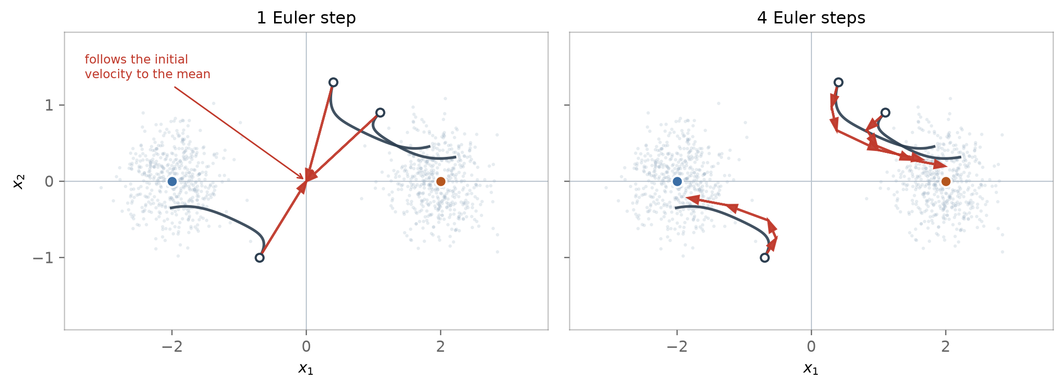
The path bows by roughly a sixth of the endpoint distance, toward the mode it eventually commits to. A single step follows only the initial velocity, which points at the dataset average instead.
Three reference trajectories (dark) with Euler steps overlaid (red); open circles mark the noise starts, faint points the data. One step leaves the data entirely for the mean at the origin; four steps begin to track the curve.
Speed — the path is not covered at a uniform rate. This part is less intuitive, so worth being explicit: even a perfectly straight path defeats a single Euler step if it is traversed at a varying rate, because the step assumes one constant velocity and will overshoot or undershoot. The mean speed across trajectories changes by about 2.7× over the journey.
The precise condition is that one Euler step is exact only when the trajectory is affine in time — a straight line covered at constant speed. Geometric straightness alone is not enough. In 2-D that is easy to picture; for images the same statement holds in pixel or latent space, where “straight” means the intermediate states are a constant-rate blend of the endpoints.
What to carry away
The network answers a narrow question: given this noisy input, what is the average clean sample consistent with it. Not a plausible sample — the average.
How much it averages over depends on noise. At \(t=1\) the answer is the dataset mean, with zero spread across 50,000 inputs; then mode-specific; then instance-specific.
The one-step collapse is not model error. With a perfect denoiser one step still lands on the mean, because a locally correct direction was extended across the whole journey. That is discretisation error — a numerical problem with numerical answers.
Error falls as \(1/n\) for this first-order sampler. Measured: roughly a factor of two per doubling of steps, once past the coarsest few. That is what makes “fifty” a budget rather than a magic number.
Sampling creates no information. The seed fixes the output; what changes is how much the denoiser can resolve.
Category first, detail later. The blob is fixed from the start — by symmetry, in this toy — while position within it takes most of the journey.
If one sentence survives: the model tells you how to move from the state you have now, and the sampler pays repeated network calls to turn those local answers into an accurate finite journey.
Where this goes next
The problem is now stated precisely: a changing velocity forces repeated evaluation, and repeated evaluation costs network calls. The next post works through four ways to reduce that cost: integrate the field better, make the field easier to integrate, learn the finite-time transport directly, or relax seed-wise transport and match the destination distribution.
Ho, Jain & Abbeel, Denoising Diffusion Probabilistic Models, 2020 — the training objective recapped above, and the variational bound that reduces to weighted squared error.