import math
import time
import torch
import torch.nn as nn
import matplotlib.pyplot as plt

torch.set_num_threads(1)
torch.manual_seed(0)
print("torch", torch.__version__)
torch 2.8.0You have an image diffusion model that works. You want video. The obvious move is to give the model a time index, train it on frames labelled with their position in the clip, and sample T of them.
It produces beautiful frames. It does not produce a video.
What comes out has an odd, specific character that anyone who has tried this recognises immediately: every individual frame is sharp and plausible, and the sequence is nonsense. The object is in a slightly different place each frame in a way no object moves. Colours shift. Identity swaps. Something occludes and comes back as something else.
If you have ever built the obvious framewise baseline, this failure is familiar: the image model is doing its job perfectly well, and nothing in the system has been asked to preserve a trajectory.
The tempting diagnosis is that the model is undertrained, or that the architecture needs temporal layers. Both may be true, but neither is the interesting part. A per-frame model can be perfect — exactly correct on every frame’s distribution — and still produce this. That is not a training failure, and no amount of per-frame capacity fixes it, because the thing it gets wrong is not a property of any frame.
This post builds that claim into something you can check.
TL;DR — A framewise generator learns the marginals \(p(x_t)\). A video is a sample from the joint \(p(x_{1:T})\). The marginals do not determine the joint, so a model can be exactly right about every frame and still produce something that is not a video. Below: two generators with provably identical per-frame distributions, one of which moves and one of which teleports; the same split reproduced with trained flow-matching models; where dependence actually enters a video architecture; and why any metric whose population value depends only on the per-frame marginals is structurally incapable of noticing the difference.
Everything here is CPU-sized. On my machine the eight toy flow models train in about a minute; the code prints its own measured time, so you can see what yours does.
What we are building. Input: nothing — this is unconditional generation. Output: a clip, a tensor of shape [T, H, W], T frames of a single moving object. The only question in this post is whether the frames that come out belong to the same trajectory.
import math
import time
import torch
import torch.nn as nn
import matplotlib.pyplot as plt
torch.set_num_threads(1)
torch.manual_seed(0)
print("torch", torch.__version__)torch 2.8.0To reason about this you want data where the difficulty is visible, not buried under texture. So: a bright blob leaves the centre of the frame in some direction and travels at constant speed.
That is deliberately the smallest thing that is still a video. It has one moving object, a persistent identity, and — the part that matters — a property that no single frame reveals. In a real clip that property is the velocity of a car, the direction a person is walking, which way a camera is panning, whose hand is entering the shot. Here it is one angle. Everything below is about what happens to that property, and a toy is the right place to watch it because in a real clip you cannot tell whether the model lost the velocity or merely rendered the texture badly.
S, T = 48, 7                                   # frame size, clip length
#     48 not 40: at 40 the last frame's blob grazes the canvas edge, and the
#     clipped tail is enough to disturb the statistics we are about to compare.
ys = torch.arange(S).float()[None, :, None]
xs = torch.arange(S).float()[None, None, :]

def render(pos, sigma=2.0):
    """Positions -> frames. Gaussian blob, so sub-pixel motion is visible."""
    y = pos[..., 0].reshape(-1)[:, None, None] + S / 2
    x = pos[..., 1].reshape(-1)[:, None, None] + S / 2
    field = torch.exp(-(((ys - y) ** 2 + (xs - x) ** 2) / (2 * sigma ** 2)))
    return field.view(*pos.shape[:-1], S, S)


def trajectories(n, gen, speed=2.4):
    """One direction per clip, held for the whole clip.

    Shapes, because they are the whole trick:
        theta                      [n, 1]      one angle per clip
        t                          [1, T]      one radius per frame
        t * sin(theta)             [n, T]      broadcast: every clip x every frame
        stack(..., dim=-1)         [n, T, 2]   a (y, x) position per frame
    The broadcast is what encodes "the direction is a property of the clip and
    the radius is a property of the frame" -- the [n,1] and [1,T] shapes meet in
    the middle. Give theta shape [n, T] instead and you get the other generator
    in this post, which is the entire subject of Act II.
    """
    theta = torch.rand(n, 1, generator=gen) * 2 * math.pi
    t = torch.arange(T).float()[None] * speed          # frame 0 at the centre
    return torch.stack([t * torch.sin(theta), t * torch.cos(theta)], dim=-1)


g = torch.Generator().manual_seed(0)
clip = render(trajectories(1, g))[0]
print(f"clip shape {tuple(clip.shape)}   (T, H, W)")
print(f"blob moves {(trajectories(1, torch.Generator().manual_seed(0))[0][1:] - trajectories(1, torch.Generator().manual_seed(0))[0][:-1]).norm(dim=-1).mean():.1f} px per frame")
clip shape (7, 48, 48) (T, H, W)
blob moves 2.4 px per framefig, axes = plt.subplots(1, T, figsize=(1.45 * T, 1.8))
for t in range(T):
axes[t].imshow(clip[t], cmap="magma", vmin=0, vmax=1)
axes[t].set_title(f"frame {t}", fontsize=9)
axes[t].set_xticks([]); axes[t].set_yticks([])
plt.tight_layout(); plt.show()
A Gaussian blob rather than a hard square, deliberately. Hard-edged shapes quantise to integer pixels, so sub-pixel motion vanishes and every temporal statistic you compute is dominated by rounding. That is a genuinely annoying half-hour to lose, and it shows up in real work too — if your evaluation clips are mostly static or your motion is smaller than a pixel, temporal metrics measure your renderer rather than your model.
Now the property that makes this toy worth using: a single frame does not determine the clip.
Look at frame 3. The blob is somewhere on a ring of radius 3 × speed around the centre. That is all frame 3 knows. It does not know which direction the blob went, because direction is a property of the sequence, and frame 3 is one frame.
So the per-frame distribution \(p(x_t)\) is a ring. It is a perfectly well-defined distribution, a model can learn it exactly, and it is the correct answer to the question “what does frame 3 look like?”
The trouble is that “what does frame 3 look like?” is the wrong question.
Here is the construction the whole post rests on. Both generators produce frames from exactly the same per-frame distribution. They differ in one line.
N = 2000
g = torch.Generator().manual_seed(0)
t_grid = torch.arange(T).float()[None] * 2.4

# COHERENT: draw one direction per clip and hold it
theta_clip = torch.rand(N, 1, generator=g) * 2 * math.pi
coherent = torch.stack([t_grid * torch.sin(theta_clip),
                        t_grid * torch.cos(theta_clip)], dim=-1)

# FRAMEWISE: draw an independent direction for every frame
theta_frame = torch.rand(N, T, generator=g) * 2 * math.pi
framewise = torch.stack([t_grid * torch.sin(theta_frame),
                         t_grid * torch.cos(theta_frame)], dim=-1)

V_coh, V_fw = render(coherent), render(framewise)
print(f"coherent  video tensor {tuple(V_coh.shape)}   (clips, T, H, W)")
print(f"framewise video tensor {tuple(V_fw.shape)}")
coherent video tensor (2000, 7, 48, 48) (clips, T, H, W)
framewise video tensor (2000, 7, 48, 48)Before any statistics, look at one clip from each. The last panel of each row overlays all frames of that clip on top of one another, which is the cheapest way to see a trajectory in a still image:
fig = plt.figure(figsize=(11, 4.4))
gs = fig.add_gridspec(2, T + 1, width_ratios=[1] * T + [1.25], wspace=0.12, hspace=0.2)

for r, (V, label, colour) in enumerate([(V_coh, "coherent", "#2E7D6F"),
                                        (V_fw, "framewise", "#B23A3A")]):
    for t in range(T):
        ax = fig.add_subplot(gs[r, t])
        ax.imshow(V[3, t], cmap="magma", vmin=0, vmax=1)
        ax.set_xticks([]); ax.set_yticks([])
        if r == 0:
            ax.set_title(f"frame {t}", fontsize=9)
        if t == 0:
            ax.set_ylabel(label, fontsize=11, color=colour, fontweight="bold")
    ax = fig.add_subplot(gs[r, T])
    ax.imshow(V[3].amax(0), cmap="magma", vmin=0, vmax=1)      # all frames at once
    ax.set_xticks([]); ax.set_yticks([])
    ax.set_title("all frames\noverlaid", fontsize=9)
    for sp in ax.spines.values():
        sp.set_edgecolor(colour); sp.set_linewidth(2.5)
plt.show()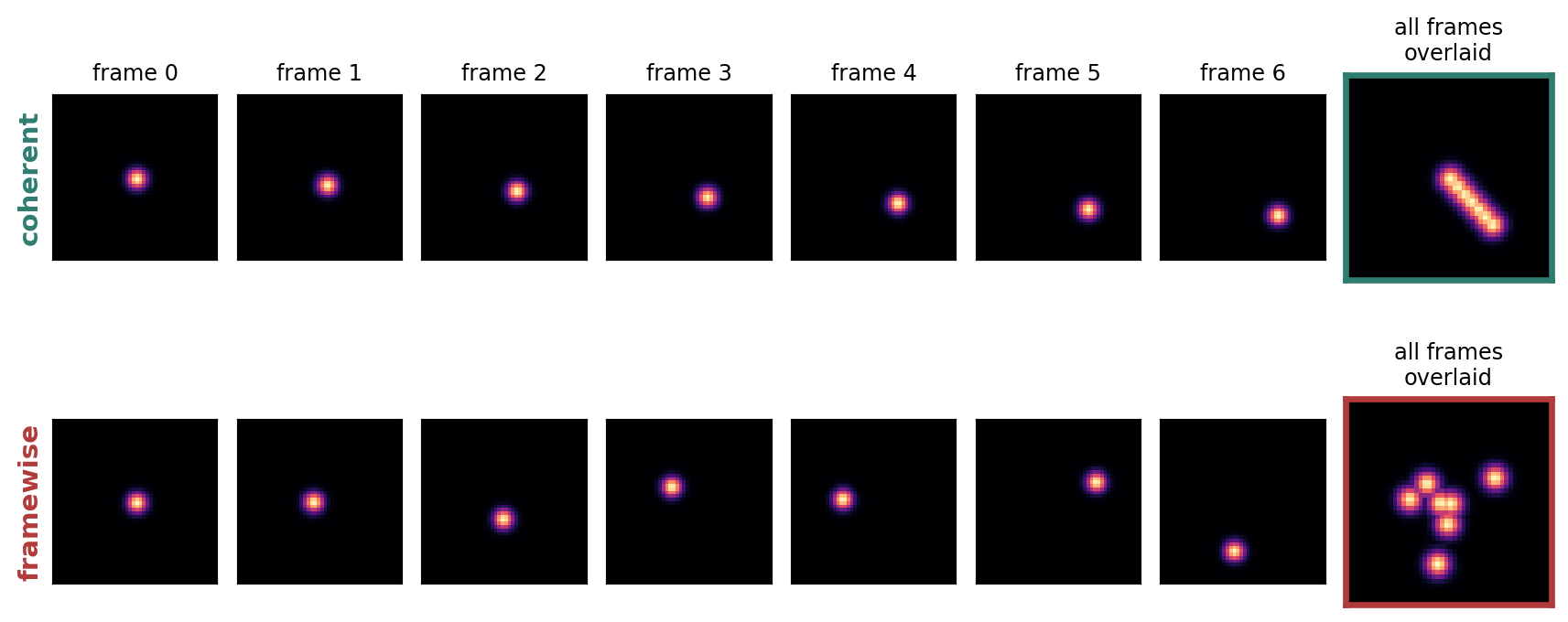
The overlay panels are the whole post in one picture. The top row traces a streak — an object that went somewhere. The bottom row is a scatter of blobs at increasing radius, which is what it looks like when something is sampled at seven different places rather than moving between them. Worth being precise about what that bottom row is: it is not a random walk. A random walk accumulates increments; here each position is drawn independently on its own expanding ring, so the increments are neither independent of position nor identically distributed. It is a sequence of independent teleports.
Now the claim that makes this interesting rather than obvious: every frame in the bottom row is drawn from exactly the same distribution as the corresponding frame in the top row.
The second one is what an independently sampled framewise generator does — no shared state, no conditioning, nothing carried between frames. It draws frame 1 from \(p(x_1)\), frame 2 from \(p(x_2)\), and so on. Every draw is from the right distribution. (Act IV comes back to why “framewise” as an architecture and “independent” as a sampling procedure are not the same claim; here they coincide because I built them to.)
That equality is not something to check empirically — it is true by construction. Frame k is a blob at radius k × speed in a uniformly random direction, in both generators, because in both cases the angle entering frame k is uniform on the circle. The per-frame population distributions are the same object.
What the numbers below show is that finite samples from those identical distributions agree up to Monte Carlo noise, which is all a finite sample can ever show:
Now, a warning about how not to check this, because the obvious check is nearly worthless. The tempting move is to compare per-frame pixel means and standard deviations. Add a third generator that is deliberately, grossly wrong — every clip travels in the same fixed direction, so the angular distribution is a point mass instead of uniform — and see whether those statistics notice:
def blobs(theta):
    return render(torch.stack([t_grid * torch.sin(theta),
                               t_grid * torch.cos(theta)], dim=-1))

V_degenerate = blobs(torch.full((N, 1), 0.7))      # every clip the same direction

print(f"{'frame':>6}{'coherent':>12}{'framewise':>12}{'degenerate':>13}   (per-frame mean)")
for k in range(T):
    print(f"{k:>6}{V_coh[:, k].mean():>12.6f}{V_fw[:, k].mean():>12.6f}"
          f"{V_degenerate[:, k].mean():>13.6f}")
print()
print(f"{'frame':>6}{'coherent':>12}{'framewise':>12}{'degenerate':>13}   (per-frame std)")
for k in [0, 3, T - 1]:
    print(f"{k:>6}{V_coh[:, k].std():>12.6f}{V_fw[:, k].std():>12.6f}"
          f"{V_degenerate[:, k].std():>13.6f}")
frame coherent framewise degenerate (per-frame mean)
0 0.010908 0.010908 0.010908
1 0.010908 0.010908 0.010908
2 0.010908 0.010908 0.010908
3 0.010908 0.010908 0.010908
4 0.010908 0.010908 0.010908
5 0.010908 0.010908 0.010908
6 0.010908 0.010908 0.010908
frame coherent framewise degenerate (per-frame std)
0 0.073042 0.073042 0.073042
3 0.073042 0.073042 0.073042
6 0.073042 0.073042 0.073042All three agree to six decimals, on every frame. The degenerate generator has a completely different marginal — all its mass on one angle instead of spread over the circle — and the per-frame mean and standard deviation cannot see it.
The reason is worth understanding rather than filing away: a Gaussian blob that stays comfortably inside the canvas carries the same total intensity and the same spatial spread wherever you put it. Translating it moves the mass without changing those summaries. Both statistics are, to the precision shown, invariant to exactly the property we care about. They would have signed off on a generator that always goes the same way.
(This is also why the canvas is 48 pixels rather than 40. At 40 the last frame’s blob grazes the edge, a sliver of mass falls off, and the three columns start disagreeing in the sixth decimal for a reason that has nothing to do with angles. A measurement artifact masquerading as a signal is worse than no measurement.)
So do not lean on a table for this at all. The equality of the marginals is a fact about the construction, not something to be estimated. In both the coherent and framewise generators, frame k is by definition a blob at radius k × speed in a uniformly random direction. The two marginals are equal as distributions. No sample size makes that more true, and a passing statistical check is not what makes it true.
That distinction matters beyond bookkeeping: it is why the claim is airtight. Any quantity that is a function of one frame’s distribution takes the same value under both generators — the histogram of pixel values, the distribution of blob positions, per-frame FID against a fixed reference set. Not approximately. Identically.
When we get to learned distributions in Act III the situation reverses: there the marginals only match approximately, so measurement becomes necessary — and we will need a statistic that can actually see the angular structure, which is exactly what the check above could not do.
temporal_diff = lambda V: ((V[:, 1:] - V[:, :-1]) ** 2).mean().item()
overlap = lambda V: (V[:, 1:] * V[:, :-1]).sum(dim=(2, 3)).mean().item()

td_c, td_f = temporal_diff(V_coh), temporal_diff(V_fw)
print(f"temporal difference energy   coherent {td_c:.6f}   framewise {td_f:.6f}"
      f"   ({td_f / td_c:.2f}x)")
print(f"consecutive-frame overlap    coherent {overlap(V_coh):.4f}"
      f"   framewise {overlap(V_fw):.4f}")
temporal difference energy coherent 0.003298 framewise 0.008535 (2.59x)
consecutive-frame overlap coherent 8.7673 framewise 2.7345Two and a half times the frame-to-frame change, and the blob in frame k+1 barely overlaps the blob in frame k. One of these is an object moving. The other is an object being re-placed from scratch seven times.
That is the whole problem, and it is worth stating in its strongest form:
Getting every frame’s distribution exactly right does not get the video right. The marginals \(p(x_1), \dots, p(x_T)\) do not determine the joint \(p(x_{1:T})\), and a video is a sample from the joint.
There is no amount of per-frame improvement that fixes this. Sharper frames, better textures, higher per-frame fidelity — all orthogonal. The framewise generator above is already optimal for any unpaired population objective that depends only on the single-frame marginal.
If you read the diffusion post, this should feel familiar. There, squared-error regression returned \(\mathbb{E}[\dot x_t \mid x_t]\), and at a point where two training pairs crossed with velocities +2 and −2 it returned their average — correctly solving a marginal regression that was not the question being asked.
Here the same word does the same damage in a different place. There, a conditional expectation averaged incompatible answers. Here, independent sampling from correct marginals destroys the dependence between them. Both are cases where each piece is right and the assembly is wrong, and both are invisible to any metric that looks at one piece at a time.
Worth being precise about the difference, though: the diffusion case was a property of what regression learns, and this one is a property of what independent sampling produces. Related in spirit, not the same theorem.
The construction above is exact, which is its strength and also a fair objection: I built both generators by hand. Does this appear when you train something?
It does, and the cheapest place to see it is in trajectory space. Strip the renderer away and model the positions directly — same flow-matching machinery as the diffusion post, so nothing here is new except what it is applied to.
def traj_samples(n, gen):
    """The same process in position space: constant speed, one random direction.

    Indexed 1..T rather than 0..T-1 as in the rendered toy. In the toy, frame 0
    sits at the centre for every clip — it is deterministic, so there is nothing
    for a generative model to learn about it. Here we drop it and model the
    frames that actually carry the ambiguity, which also keeps radius == index
    and makes the table below readable.
    """
    theta = torch.rand(n, 1, generator=gen) * 2 * math.pi
    t = torch.arange(1, T + 1).float()[None]
    return torch.stack([t * torch.sin(theta), t * torch.cos(theta)], dim=-1)


class Field(nn.Module):
    """Velocity field for flow matching. `dim` is what the model sees at once.

    Note the two different times in play. `t` indexes video frames. `tau`
    indexes the flow from noise to data. They are unrelated, and conflating
    them is the fastest way to confuse yourself here.
    """
    def __init__(self, dim, h=128):
        super().__init__()
        self.f = nn.Sequential(nn.Linear(dim + 1, h), nn.SiLU(),
                               nn.Linear(h, h), nn.SiLU(),
                               nn.Linear(h, h), nn.SiLU(),
                               nn.Linear(h, dim))

    def forward(self, x, t):
        return self.f(torch.cat([x, t.view(-1, 1)], dim=1))


def train(dim, sampler, steps=3000, bs=512, seed=0):
    """Flow matching, in six lines. The derivation is three:

        interpolate     x_tau = (1 - tau) * x + tau * z      data at 0, noise at 1
        differentiate   d x_tau / d tau = z - x              constant along the path
        regress         net(x_tau, tau)  ->  z - x           that is the whole loss

    No ODE is solved during training, which is what "simulation-free" means.
    Generation integrates the learned field backwards, from tau=1 to tau=0.
    """
    torch.manual_seed(seed)
    net = Field(dim)
    opt = torch.optim.Adam(net.parameters(), 2e-3)
    g = torch.Generator().manual_seed(1)
    for _ in range(steps):
        x = sampler(bs, g)                       # data,  tau = 0
        z = torch.randn_like(x)                  # noise, tau = 1
        tau = torch.rand(bs)                     # [bs]
        # tau[:, None] is [bs, 1] so it broadcasts across the state dimension;
        # without the None it would try to broadcast against `dim` and fail.
        x_tau = (1 - tau[:, None]) * x + tau[:, None] * z
        loss = ((net(x_tau, tau) - (z - x)) ** 2).mean()
        opt.zero_grad(); loss.backward(); opt.step()
    return net


@torch.no_grad()
def generate(net, dim, n, steps=60, seed=0):
    """Euler-integrate the field from noise (tau=1) back to data (tau=0)."""
    x = torch.randn(n, dim, generator=torch.Generator().manual_seed(seed))
    for i in range(steps):
        tau = 1 - i / steps
        x = x - (1 / steps) * net(x, torch.full((n,), tau))    # minus: tau decreasing
    return x
Two ways to use this. The joint model sees the whole trajectory as one 2T-dimensional vector. The framewise models — one per frame index — each see a single 2-D position and learn only that frame’s marginal. That is exactly what a per-frame image model does: it never sees two frames at once.
t0 = time.time()

joint_net = train(2 * T, lambda n, g: traj_samples(n, g).reshape(n, -1))
frame_nets = [train(2, lambda n, g, k=k: traj_samples(n, g)[:, k], steps=1500)
              for k in range(T)]

print(f"trained 1 joint + {T} framewise models in {time.time() - t0:.0f}s")
trained 1 joint + 7 framewise models in 11sThe k=k default argument in that lambda is not decoration. Python closures capture variables by reference, not by value, so writing lambda n, g: traj_samples(n, g)[:, k] gives every model a closure over the same k, which by training time has finished the loop and equals the last index. All seven models then train on the final frame. The symptom — seven models that behave identically — looks like a bug in the training loop rather than in the closure, and it is surprisingly easy to misdiagnose.
M = 4000
J = generate(joint_net, 2 * T, M).view(M, T, 2)
F = torch.stack([generate(frame_nets[k], 2, M, seed=k + 1) for k in range(T)], dim=1)
R = traj_samples(M, torch.Generator().manual_seed(99))

print("mean distance from origin  (truth = frame index)\n")
print(f"{'frame':>6}{'real':>10}{'joint':>10}{'framewise':>12}")
for k in range(T):
    print(f"{k+1:>6}{R[:, k].norm(dim=-1).mean():>10.3f}"
          f"{J[:, k].norm(dim=-1).mean():>10.3f}{F[:, k].norm(dim=-1).mean():>12.3f}")
mean distance from origin (truth = frame index)
frame real joint framewise
1 1.000 1.018 1.000
2 2.000 2.006 1.989
3 3.000 2.976 2.983
4 4.000 4.008 3.947
5 5.000 4.978 4.924
6 6.000 5.979 5.997
7 7.000 6.963 6.978Both match the mean radius to within about 1% at every frame. But a mean radius is one number, and matching it does not establish that the distributions match — a model can have the right average radius with badly wrong radial spread or a non-uniform angle. So check the actual 2-D distribution per frame, against the only baseline that means anything: two independent draws of real data.
def sliced_wasserstein(a, b, n_proj=128, seed=0):
    """Average 1-D Wasserstein distance over random projections of a 2-D cloud."""
    g = torch.Generator().manual_seed(seed)
    d = torch.randn(n_proj, 2, generator=g)
    d = d / d.norm(dim=1, keepdim=True)
    return ((a @ d.T).sort(0).values - (b @ d.T).sort(0).values).abs().mean().item()


R2 = traj_samples(M, torch.Generator().manual_seed(77))     # a second real draw
print(f"{'frame':>6}{'joint vs real':>16}{'framewise vs real':>20}{'real vs real':>15}")
for k in range(T):
    print(f"{k+1:>6}{sliced_wasserstein(J[:, k], R[:, k]):>16.4f}"
          f"{sliced_wasserstein(F[:, k], R[:, k]):>20.4f}"
          f"{sliced_wasserstein(R2[:, k], R[:, k]):>15.4f}")
frame joint vs real framewise vs real real vs real
1 0.0326 0.0232 0.0176
2 0.0649 0.0430 0.0353
3 0.0814 0.0548 0.0529
4 0.1016 0.1243 0.0705
5 0.1287 0.1297 0.0881
6 0.1522 0.1269 0.1058
7 0.1798 0.1910 0.1234Read the last column first: that is how far apart two real samples of the same size land, and it grows with frame index simply because the ring gets bigger. It is one finite-sample baseline, not a floor — another pair of real draws would land somewhat differently — but it sets the scale. Against it, both models sit modestly above sampling noise and, which is the point, they sit there together: same order of marginal error, no gap remotely large enough to explain what happens next.
Nor are either of them perfect. The real data has an exactly zero radial standard deviation, because every point is on the ring exactly; both models smear it. The framewise models are not secretly worse marginal learners, and the joint model is not secretly better. They differ somewhere else entirely.
Now ask whether either produced a trajectory:
def direction_consistency(X):
    """Cosine between consecutive displacements. 1 = straight, 0 = no directional persistence."""
    d = X[:, 1:] - X[:, :-1]
    c = (d[:, 1:] * d[:, :-1]).sum(-1) / (d[:, 1:].norm(dim=-1) * d[:, :-1].norm(dim=-1) + 1e-9)
    return c.mean().item()

step_size = lambda X: (X[:, 1:] - X[:, :-1]).norm(dim=-1).mean().item()

print(f"{'':<26}{'real':>10}{'joint':>10}{'framewise':>12}")
print(f"{'direction consistency':<26}{direction_consistency(R):>10.4f}"
      f"{direction_consistency(J):>10.4f}{direction_consistency(F):>12.4f}")
print(f"{'mean step size':<26}{step_size(R):>10.4f}"
      f"{step_size(J):>10.4f}{step_size(F):>12.4f}")
real joint framewise
direction consistency 1.0000 0.9848 -0.3703
mean step size 1.0000 0.9961 5.1746Numbers are one thing; draw the generated clips as paths and the difference stops needing interpretation:
fig, axes = plt.subplots(1, 3, figsize=(10.5, 3.6))
for ax, (P, label, colour) in zip(axes, [(R, "real data", "#2C4F6B"),
                                         (J, "joint model", "#2E7D6F"),
                                         (F, "framewise models", "#B23A3A")]):
    for k in range(30):
        ax.plot(P[k, :, 1], P[k, :, 0], "-o", ms=2.5, lw=0.9, alpha=0.65, color=colour)
    ax.set_title(label, fontsize=11, color=colour, fontweight="bold")
    ax.set_aspect("equal"); ax.set_xlim(-9, 9); ax.set_ylim(-9, 9)
    ax.set_xticks([]); ax.set_yticks([])
    for sp in ax.spines.values():
        sp.set_edgecolor("#DCE2E7")
plt.tight_layout(); plt.show()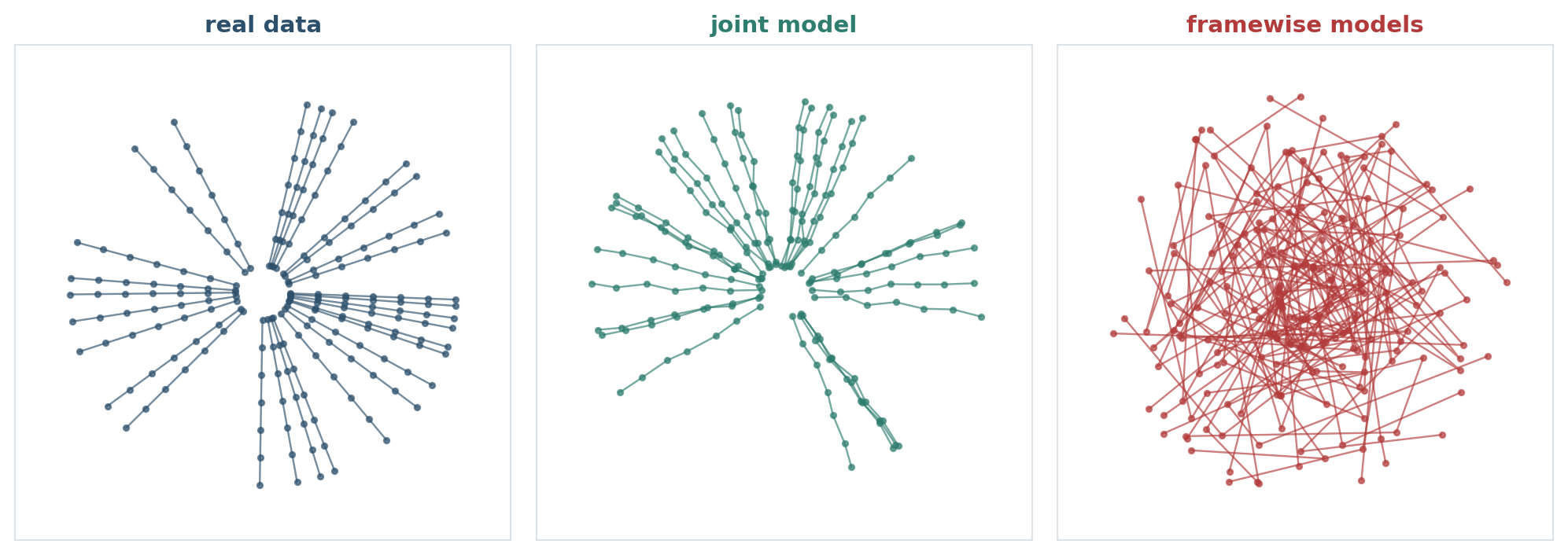
The middle panel is the process. The right panel is a scribble — and it was produced by models that, one frame at a time, are as accurate as the middle one.
The joint model reproduces the process: direction consistency 0.9848 against a true 1.0000, step size 0.9961 against 1.0000. The framewise models produce steps five times too large in directions that are anti-correlated — a negative consistency means consecutive displacements tend to point opposite ways, which is what independent draws from concentric rings look like.
Both models are doing what their objectives permit. They were asked different statistical questions. Nothing about the framewise models is broken; their per-frame distributions have marginal errors comparable to the joint model’s under the checks above. They were simply never shown two frames at the same time, so nothing in their training signal could have told them that frames are related.
The fix follows from naming the object. The independently sampled generator from Act II induces
\[p(x_{1:T}) = \prod_t p(x_t)\]
which asserts that the frames are independent. A video model needs the joint \(p(x_{1:T})\) — and by the chain rule every joint already admits a causal factorization
\[p(x_{1:T}) = p(x_1)\prod_{t=2}^{T} p(x_t \mid x_{<t})\]
so that is not a second kind of distribution. It is the same distribution written in a different order. What actually differs between systems is how the joint is parameterized and produced: denoise a whole clip at once, factorize causally and generate sequentially, or work in blocks somewhere in between. Those are modelling and systems decisions with different failure modes and different deployment properties, not different probability models.
Three computational patterns show up repeatedly. They are not a hierarchy of seriousness; they give the model different connectivity and different inductive biases, and the second and third are both joint video models. It is worth being concrete about tensor shapes, because this is where implementations quietly go wrong.
A video batch is [B, T, C, H, W]. An image model expects [B*, C, H, W].
Frame-separable computation. Flatten time into the batch: x.flatten(0, 1) giving [B*T, C, H, W]. Every frame passes through the operator without it ever seeing two frames at once. This one is a plain reshape, because [B, T, ...] → [B*T, ...] merges adjacent axes in order.
Factorized space-time. Keep the 2-D operators, and interleave operators acting along T: a 1-D convolution over time per pixel location, or attention over the T axis at each spatial position. Cheap, retrofits an existing image model, and it is what most video models built on image checkpoints do. Video LDM is the clearest worked example: spatial layers treat the B×T frames as independent images, temporal layers reshape back into video form and mix across time.
The axis juggling is where this gets quietly wrong in practice, so it is worth writing out rather than waving at. Going from “a batch of frames” to “a batch of per-pixel time series” is not a reshape:
B, T_, C, H, W = 2, 5, 3, 4, 6
video = torch.arange(B * T_ * C * H * W).float().view(B, T_, C, H, W)

spatial = video.flatten(0, 1)                                    # [B*T, C, H, W]

# WRONG: the elements are in the wrong order, and nothing complains
blind = spatial.reshape(B * H * W, C, T_)

# RIGHT: recover the axes, permute so T is last, then flatten
temporal = (spatial.view(B, T_, C, H, W)
                   .permute(0, 3, 4, 2, 1)                       # [B, H, W, C, T]
                   .reshape(B * H * W, C, T_))

back = temporal.view(B, H, W, C, T_).permute(0, 4, 3, 1, 2)      # [B, T, C, H, W]

print(f"blind reshape equals the correct transform : {torch.equal(blind, temporal)}")
print(f"round trip recovers the original video     : {torch.equal(back, video)}")
blind reshape equals the correct transform : False
round trip recovers the original video : Truereshape will happily give you a tensor of the right shape containing the wrong elements, and the failure is silent: the model trains, the loss goes down, and the temporal layer is mixing across a scrambled axis. If you take one implementation detail from this post, take this one.
Unfactorized space-time. Operators that mix space and time together: 3-D convolution, or attention over flattened space-time. More expensive, fewer structural assumptions about how the two axes interact.
Now the correction that matters, and I had this wrong in an earlier draft of this post.
It is tempting to say that flattening time into the batch asserts frame independence. It does not. Frame-separable computation means the network cannot mix information across frames given its inputs — it says nothing about whether the inputs are independent. The counterexample is sitting in Act II of this very post: the coherent generator renders each frame separately from a shared per-clip angle, and its frames are strongly dependent. Frame-separable computation, dependent frames, no temporal layer anywhere.
What produced independence in the failing case was the combination: frame-separable computation, and independently sampled per-frame state, and no shared clip-level state. Remove any one of those and the frames can be dependent again.
So dependence has three places it can live, and only one of them is a temporal layer:
c, and they remain conditionally independent. Fixed conditioning aligns semantics; it does not by itself create conditional dependence.Temporal layers are not the definition of a video model. Dependence is.
One thing this correction rules out, which is worth naming because I believed it: independent initial noise per frame does not imply independent frames. Standard joint video diffusion starts from isotropic Gaussian noise over the entire spatiotemporal tensor — every component independent, across frames included — and the denoiser maps that into a temporally correlated distribution. Independence of the prior’s components says nothing about independence of the output. Noise initialization can still matter for temporal consistency in practice, but that is a specific empirical phenomenon, not a requirement that frames share noise.
If you initialise from an image model — which nearly everyone does, because video data is scarce and image data is not — the temporal parameters are new and the spatial ones are pretrained. A common and sensible design is to arrange for the new temporal branch to contribute little or nothing at initialization, so the starting network behaves like the pretrained image model and the temporal path learns a correction from there. Video LDM does exactly this: the spatial layers stay as the pretrained image model, and the learned temporal output is mixed in through a controllable merge, with the spatial blocks optionally frozen entirely.
The specific mechanism — zero-initialized residual projections, learned gates, frozen spatial blocks — is architecture-dependent, and I would not claim a universal ranking among them. The principle is what transfers: do not let the first few hundred steps of temporal training overwrite the spatial prior you paid for.
The examples above use U-Net language because it makes the tensor operations easy to see. Modern large open video systems increasingly pair a video VAE with a diffusion or flow Transformer, but the question is unchanged: where does the model couple information across space and time?
Return to the two generators from Act II. Their per-frame distributions are equal by construction, which is not an artifact of my toy — it follows directly from how they were built. And it has an uncomfortable consequence:
State it precisely, because the sloppy version is false. Consider any metric of the form
\[M = \frac{1}{T}\sum_t M_t\big(p_{\text{gen}}(x_t),\; p_{\text{real}}(x_t)\big)\]
— a per-frame score whose population value depends only on the generated and real marginals at that frame. If the marginals match for every t, any such metric is identically blind to the temporal joint. Per-frame FID and per-frame CLIP score are of this form.
Paired metrics are a partial exception worth naming: PSNR or SSIM computed against a specific ground-truth frame depends on the coupling between prediction and reference, not on the generated marginal alone, so it is not automatically in this class. In unconditional generation there is no such pairing and the exception evaporates — but if you are doing prediction with ground truth available, per-frame PSNR is not covered by the argument above.
def mean_image_mse(V, ref):
    """A concrete member of the blind class: MSE between per-frame mean images.
    Depends only on each frame's marginal, so it is blind by construction."""
    return torch.stack([((V[:, k].mean(0) - ref[:, k].mean(0)) ** 2).mean()
                        for k in range(T)]).mean().item()


def draw(kind, n, seed):
    g = torch.Generator().manual_seed(seed)
    th = (torch.rand(n, 1, generator=g) if kind == "coherent"
          else torch.rand(n, T, generator=g)) * 2 * math.pi
    return render(torch.stack([t_grid * torch.sin(th), t_grid * torch.cos(th)], -1))


ref = draw("coherent", N, 123)
print(f"mean-image MSE    coherent {mean_image_mse(draw('coherent', N, 0), ref):.3e}"
      f"   framewise {mean_image_mse(draw('framewise', N, 0), ref):.3e}\n")

# is that difference real, or is it Monte Carlo noise? redraw each generator.
for kind in ["coherent", "framewise"]:
    vals = [mean_image_mse(draw(kind, N, s), ref) for s in [1, 2, 3]]
    print(f"  {kind:<10} across three redraws: "
          + "  ".join(f"{v:.3e}" for v in vals))

print(f"\ntemporal energy   coherent {temporal_diff(V_coh):.6f}"
      f"   framewise {temporal_diff(V_fw):.6f}")
mean-image MSE coherent 3.328e-06 framewise 2.954e-06
coherent across three redraws: 2.142e-06 2.915e-06 4.698e-06
framewise across three redraws: 3.185e-06 3.524e-06 3.933e-06
temporal energy coherent 0.003298 framewise 0.008535Read that carefully rather than eyeballing the first line. The two scores are not equal — but redrawing either generator with a different seed moves its score by more than the gap between them. The coherent generator’s own redraw range straddles the framewise redraws entirely. This metric cannot separate them, and the honest way to say so is that the difference sits inside its own sampling noise.
The temporal energy, on the same data, differs by 2.59× and is nowhere near the noise.
This is the same shape as the quantization post’s SQNR result, where an aggregate mean-squared error looked twice as bad while three quarters of the matrix had been destroyed. An aggregate is a projection, and projections lose exactly the structure they project out. Here the projection is over time.
FVD is better than per-frame FID because its features are computed over clips rather than frames, so it is at least capable of seeing temporal structure. It is still a single scalar summarising a distribution of clips, and a single scalar cannot tell you which temporal property broke.
What you actually want is a small set of measurements, each of which fails for an identifiable reason. The set below is the one I would put on the dashboard before generating a single sample.
Per-frame error — is each frame plausible in isolation? Diagnoses spatial quality only, and by the argument above, nothing else.
Temporal difference energy — \(\mathbb{E}\|x_{t+1} - x_t\|^2\) against the same statistic on real data. Too high is flicker or teleporting; too low is a model that has learned to hedge by keeping everything still, which is a real and common failure and one that a naive “smoothness is good” prior will reward.
Consecutive-frame overlap — 8.77 versus 2.73 above. Directly measures whether the thing in frame t+1 is in the neighbourhood of the thing in frame t.
Trajectory error and direction consistency — if you can extract a position, compare the path rather than the pixels. This is the metric that separated the two trained models when nothing else did.
Identity drift — does the object keep its appearance? Track a feature (colour, size, shape descriptor) across the clip and measure its variance against real clips.
Reappearance accuracy after occlusion — hide the object and bring it back. Does it return with the right identity in the right place? This is the single sharpest test of whether the model has state, and it is nearly absent from standard benchmarks.
Temporal frequency spectrum — take the Fourier transform along T per pixel and compare the average power spectrum to real video. Excess high-frequency energy can indicate flicker, and a spectrum shows it as a curve rather than a number. Under substantial motion, measure it after alignment or in a feature space — legitimate motion, camera movement and illumination changes all produce genuine high temporal frequencies.
Two caveats before you take this panel anywhere near real video. Several entries here are ground-truth-aware diagnostics for a controlled toy, not generic video metrics: consecutive-frame overlap is informative when a single object moves slowly against a static background, and misleading under fast motion or camera movement, where low overlap is correct. And each measurement indicates rather than diagnoses — high temporal-frequency energy can indicate flicker, but flicker can come from the architecture, the data, the decoder, the conditioning, the objective or the sampler, and the metric does not tell you which.
The reason for a panel rather than a single score is that these are different properties, failing independently. An aggregate tells you something is wrong; a panel tells you what to look at first.
[B, T, C, H, W] → [B*T, C, H, W] means no operator sees two frames at once; it does not make the frames independent, as the coherent generator in Act II demonstrates with a shared latent and no temporal layer at all.reshape gives you the right shape with the wrong elements. Moving from [B*T, C, H, W] to per-pixel time series needs unflatten, permute, then flatten. A blind reshape silently scrambles the axis your temporal layer is about to mix over.If one sentence survives: a video model’s job is not to make each frame likely but to make the frames jointly likely, and any metric that depends only on the per-frame marginals is structurally incapable of noticing the difference.
Everything here was 48×48 with a known renderer and one object, which is the right scale to see a mechanism and the wrong scale to say anything about real video. What carries over is the argument, not the numbers: the marginal/joint distinction does not care about resolution, and neither does the blindness of per-frame metrics. Two directions follow. Many modern high-resolution video generators do not diffuse in pixel space — they compress first and learn the dynamics in a latent video space, and that compressor is itself a temporal model whose failures are indistinguishable from dynamics failures downstream. (Pixel-space video diffusion is not obsolete; the foundational work in this area is exactly that.) And a model that generates a clip in one shot is a different object from one that extends a clip indefinitely, which is where error accumulation starts to matter.
B×T frames as independent images and temporal layers reshaping back to mix across time. It also identifies the framewise autoencoder’s decoder as a flicker source needing temporal finetuning, which is where the next post starts.