import math
import torch
import torch.nn as nn
torch.set_num_threads(1)
print("torch", torch.__version__)torch 2.8.0The run had been fine for eleven hours. Then the loss goes from 2.1 to 2.9 in one step, comes most of the way back over the next fifty, and settles a little worse than it was. Nothing crashed. No NaN. The gradient norm you logged looks unremarkable.
So you stare at the curve. And the curve, it turns out, cannot answer the question, because it is a lossy view of something much bigger: a state transition involving your data, your autograd graph, your clipping, your optimizer’s accumulated history, your gradient scaler, and your scheduler. The loss is one scalar summary of the forward pass at one point in time. It is not the thing that broke.
This post is about the five lines everybody writes and nobody reads:
optimizer.zero_grad()
loss = criterion(model(batch), target)
loss.backward()
clip_grad_norm_(model.parameters(), max_norm)
optimizer.step()
Four of those five do something materially different from what most people assume. Not subtly different — differently enough that the debugging conclusions you draw from the loss curve can be wrong in a specific, reproducible way.
TL;DR — Loss, gradient, optimizer behaviour, and whether a step actually executes are four different signals, and every link between them is looser than it looks. A finite loss can produce a non-finite gradient. Global clipping couples layers that have nothing to do with each other. Adam’s update can disagree with the gradient that produced it. And under AMP,
optimizer.step()may quietly not run while the rest of the loop carries on. So the useful debugging object is not the loss curve — it’s the transition immediately around the first bad observation, which means keeping it.
Everything below runs on CPU in a few seconds. That is deliberate: these are not exotic large-scale phenomena, they are properties of the code you already have.
import math
import torch
import torch.nn as nn

torch.set_num_threads(1)
print("torch", torch.__version__)
torch 2.8.0The mental model this invites is five statements, executed in order, each doing what its name says. Gradients are zeroed. A loss is computed. Gradients are filled in. Large ones are trimmed. Parameters move.
The real object is a state machine with branches, and the branches are invisible from the call site. Gradients may be None rather than zero, and that changes which parameters the optimizer touches. The loss may be finite while the gradients are not. Clipping may report a number that no longer describes the gradients that exist after it returns. The optimizer’s step depends on state accumulated over thousands of previous iterations. And under mixed precision, step() may decline to do anything at all.
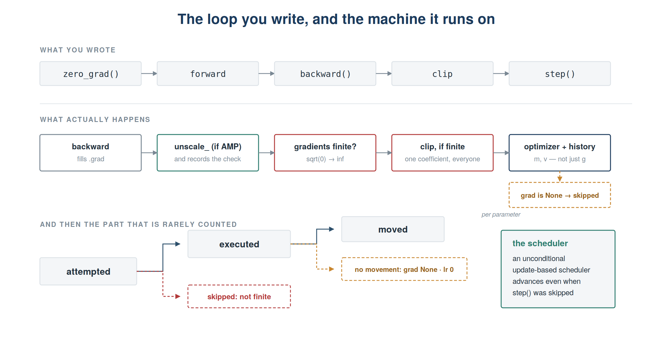
Each of the next four sections breaks one link in the chain. The pattern is the same every time: the assumption, the smallest demonstration that contradicts it, and what to do about it in production.
Start with the most common piece of hand-rolled safety code in the field — usually written just after being burned once:
loss = float("nan")

print(f"loss > 1000  -> {loss > 1000}")
print(f"loss < 1000  -> {loss < 1000}")
print(f"loss == loss -> {loss == loss}")
print(f"isfinite     -> {math.isfinite(loss)}")
loss > 1000 -> False
loss < 1000 -> False
loss == loss -> False
isfinite -> FalseEvery comparison involving NaN is False. Not just >, but < as well, and == against itself. So this guard:
if loss > SPIKE_THRESHOLD:      # never true for NaN
    skip_this_batch()
is inert for the exact condition most people wrote it to catch. It will happily catch a loss of 8000 and sail straight past a loss of NaN, forever. The code is syntactically correct, reads correctly, and does nothing.
The same is true of tensors — and this one bites harder, because the guard looks like it’s using a proper tensor predicate:
t = torch.tensor(float("nan"))
print(f"(t > 1000).item()      -> {(t > 1000).item()}")
print(f"torch.isfinite(t)      -> {torch.isfinite(t).item()}")
(t > 1000).item() -> False
torch.isfinite(t) -> FalsePractical rule: never write a NaN check as a magnitude comparison. Write if not torch.isfinite(loss): and nothing else. If you find yourself reaching for a threshold, you are testing for “too big,” which is a different and much less urgent problem.
Here is the follow-up that catches people who did write the isfinite check correctly, and checked only the loss:
x = torch.tensor(0.0, requires_grad=True)
loss = torch.sqrt(x)                       # perfectly finite
loss.backward()

print(f"forward:  sqrt(0) = {loss.item()}")
print(f"backward: d/dx    = {x.grad.item()}")
forward: sqrt(0) = 0.0
backward: d/dx = infThe forward value is 0.0. The derivative of sqrt at zero is infinite, and autograd reports it faithfully. Your loss guard passes, your gradients are already poisoned, and if that reaches a stateful optimizer unchecked it contaminates the moment buffers and everything computed from them — all without the loss ever looking wrong.
The family is the set of functions whose derivative blows up at a point where the function itself is perfectly finite: sqrt(x) and more generally \(x^\alpha\) for \(0 < \alpha < 1\) at the origin, and inverse trig at the edge of its domain — acos(1) returns 0.0 and differentiates to \(-\infty\), asin(1) returns \(\pi/2\) and differentiates to \(+\infty\).
Worth distinguishing from a neighbouring family that people lump in with it: log(0) and division by zero produce non-finite values in the forward pass, so an isfinite check on the loss does catch them. It’s the boundary-derivative cases that slip through, because there is genuinely nothing wrong with the number you checked.
PyTorch gives you a hook for this that almost nobody sets:
lin = nn.Linear(3, 3, bias=False)
lin.weight.grad = torch.full_like(lin.weight, float("inf"))

try:
    torch.nn.utils.clip_grad_norm_(lin.parameters(), 1.0, error_if_nonfinite=True)
except RuntimeError as e:
    print("raised:", str(e)[:70])

print("default for error_if_nonfinite is False — the check is opt-in")
raised: The total norm of order 2.0 for gradients from `parameters` is non-fin
default for error_if_nonfinite is False — the check is opt-inAnd there is a sharp edge behind that default, which is worth seeing before you decide to leave it off:
p = torch.nn.Parameter(torch.tensor([1.0, 2.0]))
p.grad = torch.tensor([float("inf"), 1.0])     # one component blew up

norm = torch.nn.utils.clip_grad_norm_([p], max_norm=1.0)   # default: no error
print(f"returned norm : {norm.item()}")
print(f"gradients now : {p.grad.tolist()}")
returned norm : inf
gradients now : [nan, 0.0]The clipping coefficient is max_norm / (inf + 1e-6), which is exactly 0. Multiplying through gives inf * 0 = NaN for the component that overflowed — and 1.0 * 0 = 0.0 for the component that was perfectly healthy. So the operation most people install as a safety mechanism against exploding gradients has, in the one case where a gradient truly exploded, converted a recoverable inf into an unrecoverable NaN and silently destroyed every other gradient in the model.
Gradient clipping is not a repair for non-finite gradients. It assumes they are finite and merely large.
And once you know gradients are non-finite, the next question is whose. This is the forensic move that follows:
def nonfinite_grads(model):
    """Which parameters carry non-finite gradients? Development use only."""
    return [n for n, p in model.named_parameters()
            if p.grad is not None and not torch.isfinite(p.grad).all()]

probe = nn.Sequential(nn.Linear(3, 3), nn.Linear(3, 3))
for p in probe.parameters():
    p.grad = torch.zeros_like(p)
probe[1].bias.grad = torch.full_like(probe[1].bias, float("inf"))

print("non-finite gradients in:", nonfinite_grads(probe))
non-finite gradients in: ['1.bias']That loop touches every parameter, so it is deliberately something you run after a cheap global check has already tripped — not on every step of a large model.
Note what this rules out. Checking torch.isfinite on the value clip_grad_norm_ hands back cannot help: by the time it returns, the mutation has already happened. The check has to sit between measuring and clipping, which means splitting the two operations that clip_grad_norm_ fuses:
def measure_then_clip(model, max_norm):
    """Measure first, decide, then mutate — never the other way round."""
    grads = [p.grad for p in model.parameters() if p.grad is not None]
    total = torch.nn.utils.get_total_norm(grads)
    if not torch.isfinite(total):
        return total, None                       # caller records the reason and skips
    torch.nn.utils.clip_grads_with_norm_(model.parameters(), max_norm, total)
    return total, min(1.0, max_norm / (total.item() + 1e-6))

probe = nn.Linear(2, 2)
for p in probe.parameters():
    p.grad = torch.full_like(p, float("inf"))
total, coef = measure_then_clip(probe, 1.0)
print(f"non-finite path: norm={total.item()}  coef={coef}  "
      f"grad still inf={probe.weight.grad.flatten()[0].item()}")

for p in probe.parameters():
    p.grad = torch.full_like(p, 10.0)
total, coef = measure_then_clip(probe, 1.0)
after = torch.nn.utils.get_total_norm([p.grad for p in probe.parameters()])
print(f"finite path    : norm={total.item():.3f}  coef={coef:.4f}  "
      f"post-clip={after.item():.4f}")
non-finite path: norm=inf coef=None grad still inf=inf
finite path : norm=24.495 coef=0.0408 post-clip=1.0000On the non-finite path the gradients are left exactly as they were, so whatever logs the failure still has something to look at.
Practical rule: in development, error_if_nonfinite=True is the simplest fail-fast option. If the loop needs to recover instead, measure with get_total_norm, check isfinite, and call clip_grads_with_norm_ only when the norm is finite — recording why the step was skipped rather than skipping in silence.
Now the distinction that matters most for reading curves. Take the simplest model there is, one parameter, squared error:
\[\hat y = wx, \qquad L = (\hat y - y)^2, \qquad \frac{\partial L}{\partial w} = 2(\hat y - y)\,x\]
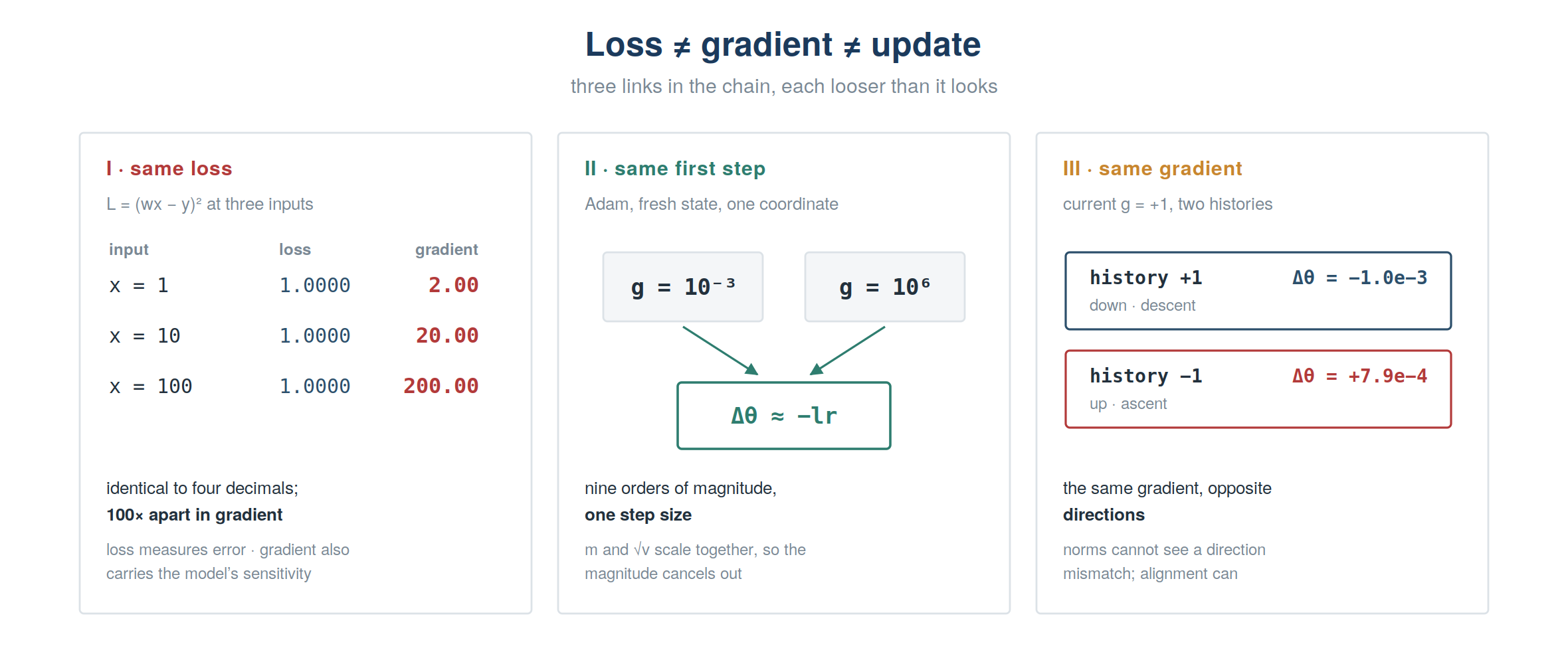
The loss depends only on the residual. The gradient depends on the residual and on the input. So two examples can have identical loss and wildly different gradients:
print(f"{'x':>8} {'y':>8} {'residual':>10} {'loss':>10} {'dL/dw':>12}")
for x, y in [(1.0, 0.0), (10.0, 9.0), (100.0, 99.0)]:
    w = torch.tensor(1.0, requires_grad=True)
    L = (w * x - y) ** 2
    L.backward()
    print(f"{x:>8.1f} {y:>8.1f} {(w.item()*x - y):>10.2f} "
          f"{L.item():>10.4f} {w.grad.item():>12.2f}")
x y residual loss dL/dw
1.0 0.0 1.00 1.0000 2.00
10.0 9.0 1.00 1.0000 20.00
100.0 99.0 1.00 1.0000 200.00Same loss to four decimals in all three rows. Gradients spanning two orders of magnitude.
This is why a smooth loss curve is not reassurance. Loss measures how wrong you are. The gradient measures how wrong you are multiplied by how sensitive the model is to the parameters at that input. A batch of long sequences, or unusually large activations, or one sample with an extreme feature scale, can produce a gradient far outside the normal range while nudging the mean loss by almost nothing.
One clarification worth making, because it is stated wrongly all the time: with reduction="mean" — the default for CrossEntropyLoss and MSELoss — the per-example gradients are averaged just like the losses are. There is no asymmetry in the averaging. The asymmetry is in what each quantity measures. A stable mean loss simply does not bound the gradient norm.
Practical rule, with the caveat that makes it honest. A high percentile of the per-example loss, logged next to the mean, finds anomalous samples; reduction="none" gives you that distribution, though not for free — a larger retained tensor, the cost of the quantile, and for token-level objectives a tensor of shape batch × sequence. Sample it or compute it on a cadence.
But per-example loss cannot detect the case just constructed, because all three rows have identical loss. Loss tails are not a proxy for gradient behaviour. Pair them with the pre-clip gradient norm, and go to per-layer contributions when that signal turns abnormal.
clip_grad_norm_ reports the pastA common training loop contains a line like this, and it is common to log the returned value as “grad norm”:
lin = nn.Linear(4, 4, bias=False)
lin.weight.grad = torch.full_like(lin.weight, 10.0)

before = lin.weight.grad.norm().item()
returned = torch.nn.utils.clip_grad_norm_(lin.parameters(), max_norm=1.0)
after = lin.weight.grad.norm().item()

print(f"norm before the call : {before:.4f}")
print(f"value returned       : {returned.item():.4f}")
print(f"norm after the call  : {after:.4f}")
norm before the call : 40.0000
value returned : 40.0000
norm after the call : 1.0000The function returns 40.0 while the gradients it just modified have norm 1.0. That is not a bug and it is not a bad design — the pre-clip norm is the diagnostically valuable number, and the post-clip norm is trivially min(max_norm, pre). But the temporal mismatch surprises people: the value describes a state that no longer exists by the time you receive it.
The consequence is that a log line reading grad_norm: 40.0 in a run with max_norm=1.0 is not evidence that clipping failed. It is evidence that clipping did a lot of work. Which is information you want — but only if you also log the clipping coefficient, because 40.0 means something very different at max_norm=1.0 than at max_norm=100.0:
\[c = \min\left(1, \frac{\texttt{max\_norm}}{\texttt{total\_norm} + 10^{-6}}\right)\]
coef = min(1.0, 1.0 / (before + 1e-6))
print(f"clipping coefficient : {coef:.6f}")
print(f"post/pre ratio       : {after / before:.6f}")
clipping coefficient : 0.025000
post/pre ratio : 0.025000Practical rule: log the pre-clip norm and the coefficient. Logging the post-clip norm alone destroys the evidence — it is pinned to max_norm on exactly the steps you most need to understand.
Here is the part of clipping that is genuinely counterintuitive. clip_grad_norm_ computes one norm, treating every gradient as though concatenated into a single vector, then multiplies all of them by the same coefficient:
model = nn.Sequential(nn.Linear(4, 4, bias=False),
                      nn.Linear(4, 4, bias=False),
                      nn.Linear(4, 4, bias=False))

for i, p in enumerate(model.parameters()):
    p.grad = torch.ones_like(p) * (0.05 if i < 2 else 100.0)  # layer 2 misbehaves

pre = [p.grad.norm().item() for p in model.parameters()]
total = torch.nn.utils.clip_grad_norm_(model.parameters(), max_norm=1.0)
post = [p.grad.norm().item() for p in model.parameters()]

print(f"total norm across all layers: {total.item():.2f}\n")
print(f"{'layer':>6} {'pre':>10} {'post':>10} {'factor':>10}")
for i, (a, b) in enumerate(zip(pre, post)):
    print(f"{i:>6} {a:>10.3f} {b:>10.5f} {b/a:>10.5f}")
total norm across all layers: 400.00
layer pre post factor
0 0.200 0.00050 0.00250
1 0.200 0.00050 0.00250
2 400.000 1.00000 0.00250Read the first two rows carefully. Layers 0 and 1 have norms of 0.2 — individually well under the max_norm of 1.0, so on their own they would not have been clipped at all. They get scaled by the same 0.0025 as the layer that actually caused the problem. Their updates for this step are effectively erased, and nothing they did caused it.
So global clipping is not “repair the exploding layer.” It is “shrink the entire proposed update direction until its total length fits.” Direction is preserved exactly; magnitude is cut for everyone. When one layer routinely dominates the norm — an embedding table early in training, an unnormalized head, a loss term with a large scale — the rest of the network is being silently starved on those steps.
Practical rule: if you clip, log which parameter group contributed most of the norm, not just the total. A run where 90% of the norm comes from one module every step is a run where every other module’s raw gradient is being scaled down without having done anything to deserve it. Under SGD that shrinks their updates directly. Under an adaptive optimizer it is less direct — as the next section shows — but it still propagates, through the optimizer state. Nothing in the loss curve will tell you either way.
Now the optimizer. Adam’s update, ignoring weight decay and \(\epsilon\), is
\[\Delta\theta = -\eta \cdot \frac{\hat m_t}{\sqrt{\hat v_t}}\]
At the very first step, with no history, \(\hat m = g\) and \(\hat v = g^2\), so the ratio is \(g/|g| = \operatorname{sign}(g)\). The magnitude cancels. Completely:
def adam_first_step(g, lr=1e-3):
    p = torch.nn.Parameter(torch.tensor([0.0]))
    opt = torch.optim.Adam([p], lr=lr)
    p.grad = torch.tensor([g])
    opt.step()
    return p.item()

for g in [1e-3, 1.0, 1e3, 1e6]:
    print(f"gradient {g:>10.0e}  ->  Δθ = {adam_first_step(g):+.6e}")
gradient 1e-03 -> Δθ = -9.999899e-04
gradient 1e+00 -> Δθ = -9.999999e-04
gradient 1e+03 -> Δθ = -9.999999e-04
gradient 1e+06 -> Δθ = -9.999999e-04A gradient of \(10^{-3}\) and a gradient of \(10^{6}\) — nine orders of magnitude apart — produce nearly the same parameter displacement. Not exactly the same: \(\epsilon\) in the denominator leaves the small-gradient case visibly short in the output above, which is itself a useful reminder that \(\epsilon\) is not decoration. But near enough that the scale has effectively been erased.
Be precise about what that establishes. At fresh state, uniformly rescaling one coordinate’s gradient largely cancels between the first- and second-moment terms of that coordinate’s update. It does not follow that any 100× spike in the global gradient norm is harmless — a norm can grow because the direction changed, or because coordinates that were quiet became active, and neither of those cancels.
What does follow is still worth carrying: current gradient magnitude need not translate proportionally into parameter displacement. And once optimizer history exists, even that simple cancellation stops being the whole story — the accumulated moments then govern both the magnitude and, as the next section shows, the direction.
It also means gradient clipping does something different under Adam than under SGD. Under plain SGD, with no momentum and no weight decay, clipping directly bounds the gradient-driven displacement. Under Adam it is not: it changes the gradient that enters the moment estimates, so its effect depends on the optimizer’s existing state and reaches both the current update and every subsequent one through \(m\) and \(v\).
A tempting next step is to conclude that Adam’s update is therefore bounded near the learning rate, with a tidy ceiling of \((1-\beta_1)/\sqrt{1-\beta_2} \approx 3.16\). That figure circulates widely and it describes exactly one situation: a gradient arriving after negligible moment state. A shaped history beats it comfortably:
def step_ratio(history, current, lr=1e-3):
    p = torch.nn.Parameter(torch.tensor([0.0]))
    opt = torch.optim.Adam([p], lr=lr)
    for g in history:
        p.grad = torch.tensor([g]); opt.step(); opt.zero_grad()
    before = p.item()
    p.grad = torch.tensor([current]); opt.step()
    return abs(p.item() - before) / lr

print(f"{'history':>34} {'|Δθ| / lr':>11}")
for label, h in [("none (fresh)", []),
                 ("500 zeros", [0.0] * 500),
                 ("2000 zeros, then 10 x 1.0", [0.0] * 2000 + [1.0] * 10),
                 ("5000 zeros, then 10 x 1.0", [0.0] * 5000 + [1.0] * 10)]:
    print(f"{label:>34} {step_ratio(h, 1.0):>11.2f}")
history |Δθ| / lr
none (fresh) 1.00
500 zeros 1.99
2000 zeros, then 10 x 1.0 6.10
5000 zeros, then 10 x 1.0 6.54Twice the supposed ceiling, from nothing more exotic than a long quiet stretch followed by a burst. The durable statement is narrower: at fresh state the gradient’s magnitude cancels out of the update, and 3.16× is not a universal bound. The step is a function of the entire gradient history, which is as much as this chapter needs from it.
This is the one that changes how you read a curve.
Adam’s numerator \(\hat m\) is an exponentially weighted average of past gradients. If that average has been pointing one way for a long time, a single opposing gradient does not immediately reverse it — the update keeps going the old way:
def adam_with_history(history, current, lr=1e-3, n=4):
    p = torch.nn.Parameter(torch.zeros(n))
    opt = torch.optim.Adam([p], lr=lr)
    for g in history:
        p.grad = torch.full((n,), g); opt.step(); opt.zero_grad()
    before = p.detach().clone()
    grad = torch.full((n,), current)
    p.grad = grad.clone(); opt.step()
    delta = p.detach() - before
    cos = torch.dot(delta, -grad) / (delta.norm() * grad.norm())
    return delta[0].item(), cos.item()

print(f"{'history':>22} {'current g':>10} {'Δθ':>13} {'cos(Δθ, −g)':>13}")
for label, h in [("fresh", []), ("30 x (+1.0)", [1.0]*30), ("30 x (−1.0)", [-1.0]*30)]:
    d, c = adam_with_history(h, +1.0)
    print(f"{label:>22} {'+1.0':>10} {d:>+13.3e} {c:>+13.4f}")
history current g Δθ cos(Δθ, −g)
fresh +1.0 -1.000e-03 +1.0000
30 x (+1.0) +1.0 -1.000e-03 +1.0000
30 x (−1.0) +1.0 +7.921e-04 -1.0000Read the last row carefully. The current gradient is positive, so descent requires moving the parameter down. The parameter moves up. The cosine between the applied update and the descent direction is \(-1\): the update is exactly anti-aligned with the gradient that produced it.
Nothing is broken. Adam is a filter over gradient history, and it is doing precisely what its update rule specifies. So for this coordinate on this step, the update is locally ascent-aligned with the current minibatch — and no quantity in the usual logging shows it. The loss is fine. The gradient norm is fine. The update magnitude is fine. Only the alignment is wrong, and alignment is rarely logged.
That is the metric this chapter is arguing for:
\[\cos(\Delta\theta,\, -g_t) = \frac{\Delta\theta \cdot (-g_t)}{\|\Delta\theta\|\,\|g_t\|}\]
Near \(+1\), the update agrees with the current batch’s descent direction. Near \(0\), it is mostly orthogonal — the optimizer is following history the current batch has no opinion about. Below \(0\), the update opposes that batch’s local descent direction, so to first order the batch’s loss is predicted to rise. Whether it actually rises over a finite step also depends on curvature and step length, which is why the experiment below measures the loss directly instead of inferring it.
A scalar toy is not evidence about real training, so let me measure it. A small MLP, a well-posed regression problem, Adam at a sane learning rate, no injected pathology — just ordinary minibatch training at four different batch sizes:
torch.manual_seed(0)
W_true = torch.randn(8, 1)

def anti_alignment_rate(batch_size, steps=400, lr=3e-3, seed=0):
    """Fraction of steps whose executed update opposes that step's own gradient."""
    torch.manual_seed(seed)
    model = nn.Sequential(nn.Linear(8, 32), nn.Tanh(), nn.Linear(32, 1))
    opt = torch.optim.Adam(model.parameters(), lr=lr)
    lossf = nn.MSELoss()
    negative, worst = 0, (1.0, None, None)

    for i in range(steps):
        X = torch.randn(batch_size, 8); y = X @ W_true
        opt.zero_grad()
        loss_before = lossf(model(X), y)
        loss_before.backward()
        g = torch.cat([p.grad.flatten() for p in model.parameters()]).clone()
        snapshot = [p.detach().clone() for p in model.parameters()]

        opt.step()

        delta = torch.cat([(p.detach() - s).flatten()
                           for p, s in zip(model.parameters(), snapshot)])
        cos = (torch.dot(delta, -g) / (delta.norm() * g.norm())).item()
        loss_after = lossf(model(X), y).item()      # same batch, after the step
        negative += cos < 0
        if cos < worst[0]:
            worst = (cos, loss_before.item(), loss_after)
    return negative / steps, worst

print(f"{'batch':>7} {'cos<0 across 4 seeds':>22} {'worst cos':>11} "
      f"{'loss on that batch':>24}")
for bs in [256, 32, 8, 2]:
    results = [anti_alignment_rate(bs, seed=s) for s in range(4)]
    rates = [r for r, _ in results]
    cos, lb, la = min((w for _, w in results))          # most anti-aligned overall
    print(f"{bs:>7} {min(rates):>10.1%} – {max(rates):<9.1%} {cos:>11.3f}   "
          f"{lb:>9.4f} -> {la:<9.4f} {'rose' if la > lb else 'fell'}")
batch cos<0 across 4 seeds worst cos loss on that batch
256 0.0% – 0.8% -0.092 0.2324 -> 0.2326 rose
32 2.0% – 3.5% -0.235 0.1102 -> 0.1113 rose
8 7.2% – 10.8% -0.588 0.0101 -> 0.0119 rose
2 7.0% – 13.8% -0.481 0.0333 -> 0.0383 roseTwo things fall out of this.
First, it is not rare and it is not a bug. In this problem, anywhere from a fraction of a percent to more than a tenth of the updates are locally anti-aligned with the current batch’s descent direction. And on the most anti-aligned transition of each run, re-evaluating that same batch after the step confirms that the finite update did in fact raise its loss — the first-order prediction holds where it was checked.
Second, smaller batches consistently produce more anti-aligned updates here. More gradient noise means the current gradient more often disagrees with the accumulated average, and momentum wins more often. The table shows seed ranges rather than single numbers, and they repay careful reading: the separation from 256 to 32 to 8 is clean, but the ranges for batch 8 and batch 2 overlap. Four seeds on a toy problem establish a direction, not a law, and any single-seed number here would have been misleading.
Be careful what you conclude from that. Alignment also depends on the learning rate, the betas, the local curvature, the phase of training, and whether the data is stationary. A shift in the alignment distribution mid-run is therefore a clue worth chasing, not a diagnosis of batch noise specifically. And this is one mechanism by which a step can hurt — not an explanation for large late-training spikes, which remain a separate question.
Practical rule: compute this periodically, not every step. It requires snapshotting parameters before the update, which at scale is expensive enough to change the thing you are measuring. A subset of layers, or a cadence you have actually timed on your own model, or capture triggered by a cheaper signal.
Under mixed precision, GradScaler multiplies the loss by a large factor so that small gradients survive fp16, then unscales before the step. If it finds inf or NaN in the gradients — which is expected and normal, it’s how the scaler calibrates — it skips optimizer.step() entirely and reduces the scale for next time.
That is correct behavior. The problem is what the rest of the loop does in the meantime:
torch.manual_seed(0)
model = nn.Linear(2, 1)
opt = torch.optim.SGD(model.parameters(), lr=0.1)
sched = torch.optim.lr_scheduler.StepLR(opt, step_size=1, gamma=0.9)
scaler = torch.amp.GradScaler(device="cpu")

attempted = moved_n = 0
print(f"{'step':>5} {'moved':>9} {'scale':>9} {'lr':>9}")
for step in range(5):
    opt.zero_grad()
    loss = model(torch.randn(4, 2)).sum()
    scaler.scale(loss).backward()

    if step == 2:                                   # stand in for an fp16 overflow
        for p in model.parameters():
            p.grad = p.grad * float("inf")

    snapshot = [p.detach().clone() for p in model.parameters()]
    scaler.step(opt)
    scaler.update()
    sched.step()                                    # unconditional — this is the bug

    attempted += 1
    moved = any(not torch.equal(a, b.detach())
                for a, b in zip(snapshot, model.parameters()))
    moved_n += moved
    print(f"{step:>5} {str(moved):>9} {scaler.get_scale():>9.0f} "
          f"{opt.param_groups[0]['lr']:>9.5f}")

print(f"\nattempted {attempted}, parameters moved {moved_n}, "
      f"scheduler advanced {attempted} -> drift {attempted - moved_n}")
step moved scale lr
0 True 65536 0.09000
1 True 65536 0.08100
2 False 32768 0.07290
3 True 32768 0.06561
4 True 32768 0.05905
attempted 5, parameters moved 4, scheduler advanced 5 -> drift 1Step 2 did not happen. The parameters are bit-identical before and after. The scale halved from 65536 to 32768, which is the scaler correctly recalibrating. And the scheduler advanced anyway, because nothing told it not to.
One skipped step is nothing. But skips can cluster early, while the scaler is still searching for a workable level — which is exactly where step-wise warmup lives. Your “step 500” is then not 500 updates, and your warmup finished before the optimizer had done the work it was warming up for.
Worth scoping: this only matters for schedules defined in optimizer-update units — step-wise warmup, cosine or linear decay counted in steps, OneCycle. An epoch-based scheduler runs on a different clock and doesn’t care, and a metric-driven one like ReduceLROnPlateau runs on a third. The bug is not “the scheduler advanced”; it is “the scheduler advanced in units of attempted steps while claiming to count updates.”
Note on this demonstration.
torch.autocast("cpu")uses bfloat16, whose exponent range matches fp32, so loss scaling is typically unnecessary there for range protection. Theinfabove is injected by hand. What these cells demonstrate isGradScaler’s control flow — faithfully, on any machine — not the frequency with which overflow occurs in a real fp16 run. Note also that the injection has to happen beforeunscale_, because that is where the scaler inspects the gradients; inject afterwards and the check has already passed, the step executes, and you have corrupted the model rather than demonstrated a skip. Real overflow frequency is a property of your model, your loss scale and your hardware — not of this cell.
So how does the loop find out? Not from the return value — scaler.step() returns the optimizer’s return value, and the common optimizers return None from step() whether it ran or not — the API permits a closure-derived value, so the return is not a reliable executed-step signal either way. Comparing parameters before and after works but costs a full copy of the model every iteration.
The clean answer is an optimizer post-step hook, which fires only when step() actually executes:
torch.manual_seed(0)
model = nn.Linear(2, 1)
opt = torch.optim.SGD(model.parameters(), lr=0.1)
sched = torch.optim.lr_scheduler.StepLR(opt, step_size=1, gamma=0.9)
scaler = torch.amp.GradScaler(device="cpu")

executed_steps = 0
def _count(optimizer, args, kwargs):
    global executed_steps
    executed_steps += 1

handle = opt.register_step_post_hook(_count)

print(f"{'step':>5} {'hook fired':>12} {'executed total':>16} {'lr':>9}")
for step in range(5):
    opt.zero_grad()
    scaler.scale(model(torch.randn(4, 2)).sum()).backward()
    if step == 2:
        for p in model.parameters():
            p.grad = p.grad * float("inf")

    before = executed_steps
    scaler.step(opt)
    scaler.update()

    if executed_steps > before:       # only advance the schedule on a real step
        sched.step()

    print(f"{step:>5} {str(executed_steps > before):>12} {executed_steps:>16} "
          f"{opt.param_groups[0]['lr']:>9.5f}")

handle.remove()
print("\nno drift: the scheduler advanced exactly as often as step() executed")
step hook fired executed total lr
0 True 1 0.09000
1 True 2 0.08100
2 False 2 0.08100
3 True 3 0.07290
4 True 4 0.06561
no drift: the scheduler advanced exactly as often as step() executedThe hook does not fire on step 2, the scheduler holds, and the learning rate now tracks executed steps rather than loop iterations.
That is a lightweight, public-API way to count executed optimizer steps. Twelve lines, no dependencies, and it turns “attempted vs executed” from a concept into a counter you can put on a dashboard.
One precision worth keeping, because it is easy to over-read the hook: it tells you step() executed, not that any parameter changed. Those are different:
lin = nn.Linear(2, 2)
opt = torch.optim.SGD(lin.parameters(), lr=0.1)
fired = []
h = opt.register_step_post_hook(lambda o, a, k: fired.append(1))

for label, setup in [("all grads None", "none"), ("lr = 0.0", "zero_lr")]:
    if setup == "none":
        opt.zero_grad(set_to_none=True)
    else:
        for q in lin.parameters():
            q.grad = torch.ones_like(q)
        opt.param_groups[0]["lr"] = 0.0

    before_n, snap = len(fired), [q.detach().clone() for q in lin.parameters()]
    opt.step()
    moved = any(not torch.equal(a, b.detach()) for a, b in zip(snap, lin.parameters()))
    print(f"{label:>16}: hook fired={len(fired) > before_n}   parameters moved={moved}")
h.remove()
all grads None: hook fired=True parameters moved=False
lr = 0.0: hook fired=True parameters moved=FalseSo the chain has three links, not two: attempted step → executed step → non-zero parameter change. The hook is a cheap answer to the middle one. The last one costs a parameter snapshot, which is why the recorder in Act II only asks it occasionally.
Practical notes. Register one counter per optimizer — GradScaler decides independently for each, so with a separate optimizer for, say, a discriminator, one can be skipped while the other steps. And if you clip or inspect gradients under AMP, you must call scaler.unscale_(optimizer) first, or you will be clipping numbers that are still multiplied by 65536 and your max_norm will mean nothing:
scaler.scale(loss).backward()
scaler.unscale_(optimizer)                     # gradients now in real units
pre_clip = clip_grad_norm_(model.parameters(), max_norm)
scaler.step(optimizer)                         # knows it was already unscaled
scaler.update()
grad is None is not grad == 0One more, and it is the shortest of the lot. The default changed to set_to_none=True some releases ago, and it has semantics:
import inspect
default = inspect.signature(torch.optim.Optimizer.zero_grad).parameters["set_to_none"].default
print(f"zero_grad default: set_to_none={default}\n")

print(f"{'set_to_none':>12} {'bias.grad':>12} {'bias moved by':>15}")
for stn in (True, False):
    lin = nn.Linear(2, 2)
    opt = torch.optim.SGD(lin.parameters(), lr=0.1, momentum=0.9, weight_decay=0.5)

    lin.weight.grad = torch.ones_like(lin.weight)      # both used once
    lin.bias.grad = torch.ones_like(lin.bias)
    opt.step()
    opt.zero_grad(set_to_none=stn)

    b0 = lin.bias.detach().clone()
    lin.weight.grad = torch.ones_like(lin.weight)      # bias NOT used this step
    opt.step()

    state = "None" if lin.bias.grad is None else "zeros"
    print(f"{str(stn):>12} {state:>12} "
          f"{(b0 - lin.bias.detach()).abs().max().item():>15.5f}")
zero_grad default: set_to_none=True
set_to_none bias.grad bias moved by
True None 0.00000
False zeros 0.14653A parameter whose .grad is None is skipped by the optimizer. A parameter whose .grad is a tensor of zeros is processed: existing momentum still carries it, and SGD’s weight-decay term still acts on it. Zero gradient does not mean zero update. (Note that SGD’s weight_decay is the conventional L2 term folded into the gradient — AdamW’s decoupled decay is a different mechanism, and it moves a zero-gradient parameter too.)
| after backward | optimizer behaviour |
|---|---|
p.grad is None |
parameter skipped entirely |
p.grad is all zeros |
processed; momentum and weight decay may still move it |
The exact displacement depends on your optimizer, learning rate, momentum state and decay, so don’t memorize the number above — memorize the distinction. It matters wherever parameters are conditionally used: mixture-of-experts routing, multi-task heads where one task is absent from a batch, frozen-then-unfrozen modules, and any branch that some batches don’t take. Switching set_to_none changes whether those parameters drift on the steps they weren’t used.
Now put the timeline together, because this is what makes the whole chapter actionable:
                    batch B_t
                        ↓
  parameters θ_t  →  loss L_t  →  gradient g_t     ← L_t is what you logged
         ↑                             ↓
  previous transition          clip, optimizer, scaler
                                       ↓
                                parameters θ_{t+1}
The loss you logged at step \(t\) was computed with \(\theta_t\), before that step’s update ran. So a bad \(L_t\) cannot have been caused by the optimizer step that follows it. That single fact eliminates the thing most people look at first.
What it leaves is \(L_t = F(\theta_t,\, B_t,\, s_t,\, \xi_t)\) — parameters, batch, and two things people forget: \(s_t\), the mutable state carried in the model (normalization running statistics, any custom module that accumulates), and \(\xi_t\), the stochastic state (dropout masks, augmentation, dataloader shuffling). The first two suspects are the state entering the forward and the batch being evaluated; the other two are why a “reproduce it” attempt sometimes doesn’t.
That fork is the whole diagnosis. When you see a spike at step 12,047, there are two objects worth having: the transition from 12,046 into 12,047 — pre-clip norm, whether the step executed, alignment, learning rate, whether a checkpoint had just been resumed — and the identity of batch 12,047, so you can feed it again and see whether the loss is high on it for any set of weights. On which: a batch ID makes replay possible, not automatic. A faithful replay also needs the parameters from that step, the model’s mutable buffers, and the RNG state — which is a good argument for the checkpoint discussion at the end of this chapter, and a good reason to record the seed alongside the batch ID.
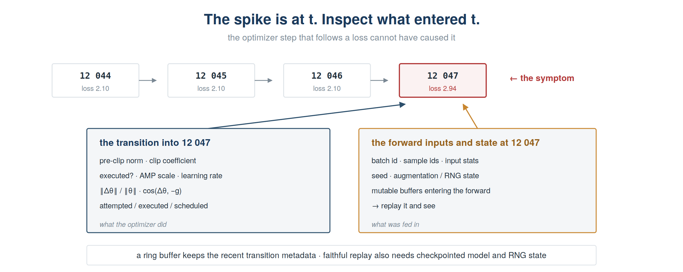
And there is the practical problem: by the time you notice, that transition is gone. You logged a scalar.
A dashboard shows you the present. A spike is evidence about the recent past. So the right instrument is a small ring buffer that keeps the last few dozen transitions and persists itself when something trips.
The design constraint that matters is cost. Some of these fields are free because you’re already computing them; others require extra work per step. Separate them:
Cheap, always on — raw unsmoothed loss, a finite flag, learning rate, AMP scale, attempted and executed counters, batch identifiers, and the pre-clip norm and clipping coefficient if you were clipping anyway.
Periodic or anomaly-triggered — per-example loss percentiles, per-layer norm contributions, update-to-weight ratio, and the update–gradient cosine. These need parameter snapshots or extra reductions. Compute them on a cadence or behind an anomaly trigger, and pick that cadence only after measuring its overhead on your own model.
from collections import deque

class FlightRecorder:
    """Ring buffer of recent training transitions, dumped when something trips.

    Cheap fields are recorded every step. Expensive ones (those needing a
    parameter snapshot) are recorded on an interval.
    """

    def __init__(self, capacity=32, deep_every=10):
        self.buf = deque(maxlen=capacity)
        self.deep_every = deep_every
        self.attempted = 0
        self.executed = 0
        self.sched_n = 0

    def snapshot(self, model):
        """Call before optimizer.step() on deep steps; returns None otherwise."""
        if self.attempted % self.deep_every:
            return None
        return [p.detach().clone() for p in model.parameters()]

    def record(self, *, step, loss, model, snapshot=None, grad=None,
               pre_clip=None, clip_coef=None, lr=None, scale=None,
               executed=None, scheduled=False, batch_id=None):
        self.attempted += 1
        if executed:
            self.executed += 1
        if scheduled:
            self.sched_n += 1

        row = dict(step=step,
                   loss=float(loss),
                   finite=bool(torch.isfinite(torch.as_tensor(loss))),
                   pre_clip=pre_clip, clip_coef=clip_coef,
                   lr=lr, scale=scale, executed=executed,
                   attempted_n=self.attempted, executed_n=self.executed,
                   sched_n=self.sched_n,
                   batch_id=batch_id, ratio=None, cos=None)

        if snapshot is not None:                       # the expensive half
            delta = torch.cat([(p.detach() - s).flatten()
                               for p, s in zip(model.parameters(), snapshot)])
            before = torch.cat([s.flatten() for s in snapshot])   # pre-update norm
            row["ratio"] = (delta.norm() / (before.norm() + 1e-12)).item()
            if grad is not None and delta.norm() > 0:
                row["cos"] = (torch.dot(delta, -grad) /
                              (delta.norm() * grad.norm() + 1e-12)).item()
        self.buf.append(row)

    @staticmethod
    def clip_coefficient(total_norm, max_norm):
        """None when the norm is non-finite — min(1, nan) silently returns 1."""
        if not math.isfinite(total_norm):
            return None
        return min(1.0, max_norm / (total_norm + 1e-6))

    def dump(self, n=6, clocks=False):
        cols = f"{'step':>5} {'loss':>9} {'fin':>4} {'preclip':>9} {'coef':>7}"
        cols += (f" {'lr':>8} {'scale':>8} {'att/exe/sch':>13}" if clocks
                 else f" {'exe':>4}")
        print(cols + f" {'ratio':>9} {'cos':>7}")
        for r in list(self.buf)[-n:]:
            f = lambda v, sp: (sp.format(v) if v is not None else "  -")
            line = (f"{r['step']:>5} {r['loss']:>9.4f} {str(r['finite'])[0]:>4} "
                    f"{f(r['pre_clip'], '{:>9.3f}'):>9} "
                    f"{f(r['clip_coef'], '{:>7.4f}'):>7}")
            if clocks:
                line += (f" {f(r['lr'], '{:>8.5f}'):>8} {f(r['scale'], '{:>8.0f}'):>8}"
                         f" {r['attempted_n']:>3}/{r['executed_n']:>3}/{r['sched_n']:<3}")
            else:
                line += f" {str(r['executed'])[0]:>4}"
            print(line + f" {f(r['ratio'], '{:>9.2e}'):>9} "
                         f"{f(r['cos'], '{:>+7.3f}'):>7}")
Two design decisions worth calling out. The loss stored is raw, never the smoothed value you plot — smoothing is a display choice and it destroys exactly the single-step evidence you need. And batch_id is not decoration: if the recorder tells you the transition into step 12,047 was anomalous, the very next thing you want is to re-run that batch, and you can only do that if you know which one it was.
And a scoping warning, because this is teaching code. [p.detach().clone() for p in model.parameters()] is fine for a model of this size and completely inappropriate for a large one — at billions of parameters it is not merely “not free,” it may not fit, and the memory pressure alone can change what you were trying to measure. In a real system: snapshot a fixed subset of layers, or accumulate the statistics inside an optimizer hook where the deltas are already available, or capture deeply only after a cheap always-on signal has already tripped. Pick the cadence by measuring its overhead on your own model, not by copying a number out of a blog post.
Now use it. A normal run, small batches, deliberately noisy — and we go looking for the most anti-aligned transition it produced:
torch.manual_seed(3)
model = nn.Sequential(nn.Linear(8, 32), nn.Tanh(), nn.Linear(32, 1))
opt = torch.optim.Adam(model.parameters(), lr=3e-3)
lossf = nn.MSELoss()
rec = FlightRecorder(capacity=64, deep_every=1)

TRIP = -0.30                                   # dump the buffer when alignment goes bad

for step in range(400):
    X = torch.randn(4, 8); y = X @ W_true
    opt.zero_grad()
    loss = lossf(model(X), y)
    loss.backward()

    g = torch.cat([p.grad.flatten() for p in model.parameters()]).clone()
    pre_clip = torch.nn.utils.clip_grad_norm_(model.parameters(), 1.0)
    snap = rec.snapshot(model)
    opt.step()

    rec.record(step=step, loss=loss.item(), model=model, snapshot=snap, grad=g,
               pre_clip=pre_clip.item(),
               clip_coef=rec.clip_coefficient(pre_clip.item(), 1.0),
               lr=opt.param_groups[0]["lr"], executed=True, batch_id=step)

    cos = rec.buf[-1]["cos"]
    if cos is not None and cos < TRIP:
        after = lossf(model(X), y).item()          # same batch, after the step
        print(f"tripped at step {step}: cos = {cos:+.3f}")
        print(f"loss on batch {step}: {loss.item():.5f} -> {after:.5f} "
              f"({'rose' if after > loss.item() else 'fell'})\n")
        rec.dump(5)
        break
tripped at step 123: cos = -0.382
loss on batch 123: 0.28032 -> 0.29854 (rose)
step loss fin preclip coef exe ratio cos
119 0.3402 T 3.836 0.2607 T 6.43e-03 +0.631
120 0.0300 T 0.712 1.0000 T 6.32e-03 +0.521
121 0.2044 T 1.997 0.5008 T 5.57e-03 +0.210
122 0.0984 T 1.411 0.7087 T 4.52e-03 -0.258
123 0.2803 T 2.937 0.3404 T 3.41e-03 -0.382Nothing here is broken. There is no injected pathology and no adversarial construction — just Adam, small batches, and momentum. The recorder tripped on its own, and the loss on that batch went up after the step that batch paid for.
Now read the cos column upward from the trip. It does not jump; it slides — positive and healthy, then weakening, then through zero, then negative for two consecutive steps. The optimizer was progressively disagreeing with the incoming batches for several steps before the trip fired.
And look at what the other columns were doing meanwhile. The pre-clip norm on the tripped step sits squarely inside the range of its neighbours. The update ratio is, if anything, smaller than the preceding steps. Neither column flags anything. If pre-clip norm and update magnitude were your only two signals — and for most training loops they are — this transition is completely invisible. The alignment column is the only one carrying the information. That is the whole argument for paying to compute it.
The second replay is the AMP failure with the recorder attached, so you can see what it looks like in the log rather than in a narrative:
torch.manual_seed(0)
model = nn.Linear(4, 1)
opt = torch.optim.SGD(model.parameters(), lr=0.05, momentum=0.9)
sched = torch.optim.lr_scheduler.StepLR(opt, step_size=1, gamma=0.95)
scaler = torch.amp.GradScaler(device="cpu")
rec = FlightRecorder(capacity=16, deep_every=1)

executed_flag = {"v": False}
h = opt.register_step_post_hook(lambda o, a, k: executed_flag.__setitem__("v", True))

for step in range(6):
    X = torch.randn(16, 4); y = X.sum(1, keepdim=True)
    opt.zero_grad()
    loss = nn.functional.mse_loss(model(X), y)
    scaler.scale(loss).backward()

    if step in (2, 3):                                # stand-in for fp16 overflow,
        for p in model.parameters():                  # injected while still scaled
            p.grad = p.grad * float("inf")

    lr_used = opt.param_groups[0]["lr"]               # the LR THIS step runs under
    scale_used = scaler.get_scale()                   # ...and the scale it runs under
    scaler.unscale_(opt)                              # this is where the scaler looks
    g = torch.cat([p.grad.flatten() for p in model.parameters()]).clone()

    # measure first, mutate only if the measurement is usable
    grads = [p.grad for p in model.parameters() if p.grad is not None]
    pre_clip = torch.nn.utils.get_total_norm(grads)
    if torch.isfinite(pre_clip):
        torch.nn.utils.clip_grads_with_norm_(model.parameters(), 1.0, pre_clip)
        coef = min(1.0, 1.0 / (pre_clip.item() + 1e-6))
    else:
        coef = None                                   # do NOT clip inf into NaN
    snap = rec.snapshot(model)

    executed_flag["v"] = False
    scaler.step(opt)
    scaler.update()
    sched.step()                                      # NAIVE: advances regardless

    rec.record(step=step, loss=loss.item(), model=model, snapshot=snap, grad=g,
               pre_clip=pre_clip.item(), clip_coef=coef,
               lr=lr_used, scale=scale_used,        # not the post-sched.step() value
               executed=executed_flag["v"], scheduled=True, batch_id=step)

h.remove()
rec.dump(6, clocks=True)
print(f"\nattempted {rec.attempted} / executed {rec.executed} / "
      f"scheduled {rec.sched_n}   -> drift {rec.sched_n - rec.executed}")
step loss fin preclip coef lr scale att/exe/sch ratio cos
0 3.1823 T 2.835 0.3527 0.05000 65536 1/ 1/1 7.77e-02 +1.000
1 7.9891 T 7.555 0.1324 0.04750 65536 2/ 2/2 1.43e-01 +0.983
2 4.1737 T inf - 0.04512 65536 3/ 2/3 0.00e+00 -
3 4.1906 T inf - 0.04287 32768 4/ 2/4 0.00e+00 -
4 5.7833 T 6.435 0.1554 0.04073 16384 5/ 3/5 1.68e-01 +0.842
5 5.6942 T 5.708 0.1752 0.03869 16384 6/ 4/6 2.19e-01 +0.965
attempted 6 / executed 4 / scheduled 6 -> drift 2This loop advances the scheduler unconditionally — the way almost every training script does — and the att/exe/sch column is the whole diagnosis. Three counters that should march together, visibly coming apart at step 2 and never re-converging. The pre-clip norm is non-finite on exactly those steps, the clipping coefficient correctly declines to report a number rather than printing a misleading 1.0, the update ratio is zero because the parameters genuinely did not move, and the learning rate kept decaying through all of it.
Notice also what didn’t happen: the loss stays finite throughout. The scaler did its job — it saw non-finite gradients, declined to apply them, and the model survived. This is the part people misread most often. The skipped steps are not the failure; they are the mechanism working. The failure is the schedule advancing as though they hadn’t been skipped, and the only reason it is visible here is that we counted the two clocks separately.
The fix is the hook from Act I — wrap sched.step() in if executed_flag["v"]: and the third counter tracks the second. One line, once you know which line.
Two things in that loop are deliberate, and both come from earlier sections.
torch.nn.utils.get_total_norm measures without touching anything; clip_grads_with_norm_ does the mutation. Splitting them lets the loop check isfinite on the norm before deciding to clip — because clip_grad_norm_, which does both at once, would have turned those inf gradients into NaN and zeroed every healthy gradient alongside them. The step was going to be skipped anyway, so nothing would have broken; but a recorder that corrupts the evidence it is recording is not a recorder. This is the production shape of the safety rule from Act I.
A third detail is easy to get wrong and quietly ruins the log. The learning rate is captured before sched.step() runs. Read it afterwards and you record the rate for the next transition, not the one you are describing — in a chapter arguing that telemetry exists to reconstruct the transition that happened, logging the wrong side of the scheduler would be a small disaster.
The other is the ordering, which is load-bearing: unscale_ comes before clip_grad_norm_, which comes before scaler.step(). Get that wrong and the pre-clip norm you record is too large by whatever the loss scale happens to be at that moment — a moving target, since the scaler adapts it — so your clipping threshold is meaningless, and the log you were relying on to debug the run is itself wrong.
With those signals in the recorder, the diagnosis becomes a lookup rather than a guess:
| observation | first place to look |
|---|---|
| Loss non-finite | inputs and forward activations; arithmetic that overflows in the forward — log(0), division by zero, sqrt of a negative |
| Loss finite, gradients non-finite | a boundary derivative where the forward was fine — sqrt(0), acos(1); also AMP overflow and custom backward functions |
| Large pre-clip norm, tiny clip coefficient | which parameter group contributed the norm; an anomalous batch |
| Ordinary gradient, abnormal update ratio or cosine | optimizer state, learning-rate change, a checkpoint resume |
| No optimizer attempt this microstep | gradient-accumulation boundary, or intentional gating |
Attempted, but step() never executed |
AMP skipping on non-finite gradients |
step() executed, but nothing moved |
grad is None for that parameter, zero LR, or an update that rounded away |
| Loss spike with no abnormal transition | a data outlier, a distribution boundary, or logging misalignment |
Then, whichever row you land on: inspect the transition before the first bad observation, not the transition it appeared in.
The last row deserves its own note, because it is the one most often skipped. If the transition genuinely looks normal, believe the instrument: a clean parameter transition shifts suspicion toward the current batch, the stochastic state, the mutable buffers, or a mismatch between what was logged and what was assumed. None of those is fixed by tuning the learning rate.
Everything above is single-process and CPU, and it stays honest by construction. Distributed training adds failure modes that none of these cells can reproduce, and here I am reporting operational experience rather than measurement — treat it accordingly.
The one thing that is documented rather than anecdotal: with a sharded model under FSDP, torch.nn.utils.clip_grad_norm_ is not the right call, because each rank holds only a shard of each gradient and the true norm spans all of them. FSDP provides its own clip_grad_norm_, and it must be called on every rank, because it performs a collective.
The rest is what tends to bite:
no_sync, sharded, pipeline or model-parallel setups, ranks can end up making independent decisions about whether to skip a step. Decide deliberately whether skip decisions are collective; don’t let it be an accident of where the check happens to sit.NaN is False, including <. Use torch.isfinite and nothing else.sqrt(0) is finite going forward and infinite coming back. error_if_nonfinite=True exists and is off by default.clip_grad_norm_ returns the pre-clip norm, after having already modified the gradients. Log it together with the clipping coefficient; the post-clip norm alone tells you nothing. And it is not a repair for non-finite gradients — it turns an inf into a NaN and zeros every other gradient in the model.GradScaler skips silently; register_step_post_hook tells you whether step() ran; only a parameter delta tells you whether anything changed. Gate the scheduler on the second.grad is None and grad == 0 are different to the optimizer. One is skipped, the other is processed and may still move.If one sentence survives: the loss curve is a lossy view of a stateful transition — record enough to reconstruct the transition, and the spike stops being a mystery.
The instability discussed here is mostly about state and control flow. For the arithmetic underneath it — where the non-finite values are actually born, and why a mathematically correct formula returns the wrong answer — see numerical stability. For the optimizer internals this chapter assumes, optimizers from scratch derives the moments and the decoupling that makes AdamW different from Adam with L2.
torch.optim.Optimizer.zero_grad — the set_to_none default and its semantics.torch.nn.utils.clip_grad_norm_ — total-norm computation, in-place modification, error_if_nonfinite.torch.optim.Optimizer.register_step_post_hook — the executed-step signal; it runs after step(), which is not the same as a parameter having changed.unscale_ ordering, skipped steps, per-optimizer behaviour.FullyShardedDataParallel — why sharded models need FSDP’s own gradient clipping.